General workflow demonstration

Setup and configuration

# # If you have JupyterLab, you will need to install the JupyterLab extension:
# # !jupyter labextension install @jupyter-widgets/jupyterlab-manager jupyter-leaflet

# On a normal notebook server, the extension needs only to be enabled
# !jupyter nbextension enable --py --sys-prefix ipyleaflet

import os

os.environ["USE_PYGEOS"] = "0"  # force use Shapely with GeoPandas

import ipyleaflet
from birdy import WPSClient
from siphon.catalog import TDSCatalog

# we will use these coordinates later to center the map on Canada
canada_center_lat_lon = (52.4292, -93.2959)

PAVICS URL configuration

# Ouranos production server
pavics_url = "https://pavics.ouranos.ca"

finch_url = os.getenv("WPS_URL")
if not finch_url:
    finch_url = f"{pavics_url}/twitcher/ows/proxy/finch/wps"

Getting user input from a map widget

Notes about ipyleaflet

ipyleaflet is a “A Jupyter / Leaflet bridge enabling interactive maps in the Jupyter notebook”

This means that the interactions with graphical objects on the map and in python are synchronized. The documentation is at: https://ipyleaflet.readthedocs.io

leaflet_map = ipyleaflet.Map(
    center=canada_center_lat_lon,
    basemap=ipyleaflet.basemaps.Esri.WorldTerrain,
    zoom=4,
)

initial_marker_location = canada_center_lat_lon
marker = ipyleaflet.Marker(location=initial_marker_location, draggable=True)
leaflet_map.add_layer(marker)

leaflet_map

If you move the marker on the map, it will update the marker.location variable. Also, if you update marker.location manually (marker.location = (45.44, -90.44)) it will also move on the map.

marker.location = (45.55, -72.44)

print(initial_marker_location)
print(marker.location)

(52.4292, -93.2959)
[45.55, -72.44]

Helper function to get user input

import ipyleaflet
import ipywidgets as widgets
from IPython.display import display


def get_rectangle():
    canada_center = (52.4292, -93.2959)
    m = ipyleaflet.Map(
        center=canada_center,
        basemap=ipyleaflet.basemaps.Esri.WorldTerrain,
        zoom=4,
    )

    # Create a new draw control
    draw_control = ipyleaflet.DrawControl()

    # disable some drawing inputs
    draw_control.polyline = {}
    draw_control.circlemarker = {}
    draw_control.polygon = {}

    draw_control.rectangle = {
        "shapeOptions": {
            "fillColor": "#4ae",
            "color": "#4ae",
            "fillOpacity": 0.3,
        }
    }

    output = widgets.Output(layout={"border": "1px solid black"})

    rectangle = {}

    # set drawing callback
    def callback(control, action, geo_json):
        if action == "created":
            # note: we can't close the map or remove it from the output
            # from this callback. The map keeps the focus, and the
            # jupyter keyboard input is messed up.
            # So we set it very thin to make it disappear :)
            m.layout = {"max_height": "0"}
            with output:
                print("*User selected 1 rectangle*")
                rectangle.update(geo_json)

    draw_control.on_draw(callback)

    m.add_control(draw_control)

    with output:
        print("Select a rectangle:")
        display(m)

    display(output)

    return rectangle

The user wants to select a rectangle on a map, and get a GeoJSON back

# NBVAL_IGNORE_OUTPUT


rectangle = get_rectangle()

#  GeoJSON with custom style properties
if not len(rectangle):
    # Use the default region of Greater Montreal Area
    rectangle = {
        "type": "Feature",
        "properties": {
            "style": {
                "stroke": True,
                "color": "#4ae",
                "weight": 4,
                "opacity": 0.5,
                "fill": True,
                "fillColor": "#4ae",
                "fillOpacity": 0.3,
                "clickable": True,
            }
        },
        "geometry": {
            "type": "Polygon",
            "coordinates": [
                [
                    [-74.511948, 45.202296],
                    [-74.511948, 45.934852],
                    [-72.978537, 45.934852],
                    [-72.978537, 45.202296],
                    [-74.511948, 45.202296],
                ]
            ],
        },
    }
rectangle

{'type': 'Feature',
 'properties': {'style': {'stroke': True,
   'color': '#4ae',
   'weight': 4,
   'opacity': 0.5,
   'fill': True,
   'fillColor': '#4ae',
   'fillOpacity': 0.3,
   'clickable': True}},
 'geometry': {'type': 'Polygon',
  'coordinates': [[[-74.511948, 45.202296],
    [-74.511948, 45.934852],
    [-72.978537, 45.934852],
    [-72.978537, 45.202296],
    [-74.511948, 45.202296]]]}}

Get the maximum and minimum bounds

import geopandas as gpd

rect = gpd.GeoDataFrame.from_features([rectangle])
bounds = rect.bounds
bounds

	minx	miny	maxx	maxy
0	-74.511948	45.202296	-72.978537	45.934852

Calling wps processes

For this example, we will subset a dataset with the user-selected bounds, and launch a heat wave frequency analysis on it.

finch = WPSClient(finch_url, progress=False)

help(finch.subset_bbox)

Help on method subset_bbox in module birdy.client.base:

subset_bbox(resource=None, lon0=0.0, lon1=360.0, lat0=-90.0, lat1=90.0, start_date=None, end_date=None, variable=None) method of birdy.client.base.WPSClient instance
    Return the data for which grid cells intersect the bounding box for each input dataset as well as the time range selected.
    
    Parameters
    ----------
    resource : ComplexData:mimetype:`application/x-netcdf`, :mimetype:`application/x-ogc-dods`
        NetCDF files, can be OPEnDAP urls.
    lon0 : float
        Minimum longitude.
    lon1 : float
        Maximum longitude.
    lat0 : float
        Minimum latitude.
    lat1 : float
        Maximum latitude.
    start_date : string
        Initial date for temporal subsetting. Can be expressed as year (%Y), year-month (%Y-%m) or year-month-day(%Y-%m-%d). Defaults to first day in file.
    end_date : string
        Final date for temporal subsetting. Can be expressed as year (%Y), year-month (%Y-%m) or year-month-day(%Y-%m-%d). Defaults to last day in file.
    variable : string
        Name of the variable in the NetCDF file.
    
    Returns
    -------
    output : ComplexData:mimetype:`application/x-netcdf`
        netCDF output
    ref : ComplexData:mimetype:`application/metalink+xml; version=4.0`
        Metalink file storing all references to output files.

Subset tasmin and tasmax datasets

# gather data from the PAVICS data catalogue
catalog = "https://pavics.ouranos.ca/twitcher/ows/proxy/thredds/catalog/datasets/gridded_obs/catalog.xml"  # TEST_USE_PROD_DATA

cat = TDSCatalog(catalog)
data = [
    cat.datasets[d].access_urls["OPENDAP"] for d in cat.datasets if "nrcan_v2" in d
][0]
data

'https://pavics.ouranos.ca/twitcher/ows/proxy/thredds/dodsC/datasets/gridded_obs/nrcan_v2.ncml'

# NBVAL_IGNORE_OUTPUT

# If we want a preview of the data, here's what it looks like:
import xarray as xr

ds = xr.open_dataset(data, chunks="auto")
ds

<xarray.Dataset> Size: 162GB
Dimensions:  (lat: 510, lon: 1068, time: 24837)
Coordinates:
  * lat      (lat) float32 2kB 83.46 83.38 83.29 83.21 ... 41.21 41.12 41.04
  * lon      (lon) float32 4kB -141.0 -140.9 -140.8 ... -52.21 -52.13 -52.04
  * time     (time) datetime64[ns] 199kB 1950-01-01 1950-01-02 ... 2017-12-31
Data variables:
    tasmin   (time, lat, lon) float32 54GB dask.array<chunksize=(3375, 69, 144), meta=np.ndarray>
    tasmax   (time, lat, lon) float32 54GB dask.array<chunksize=(3375, 69, 144), meta=np.ndarray>
    pr       (time, lat, lon) float32 54GB dask.array<chunksize=(3375, 69, 144), meta=np.ndarray>
Attributes: (12/15)
    Conventions:          CF-1.5
    title:                NRCAN ANUSPLIN daily gridded dataset : version 2
    history:              Fri Jan 25 14:11:15 2019 : Convert from original fo...
    institute_id:         NRCAN
    frequency:            day
    abstract:             Gridded daily observational dataset produced by Nat...
    ...                   ...
    dataset_id:           NRCAN_anusplin_daily_v2
    version:              2.0
    license_type:         permissive
    license:              https://open.canada.ca/en/open-government-licence-c...
    attribution:          The authors provide this data under the Environment...
    citation:             Natural Resources Canada ANUSPLIN interpolated hist...

xarray.Dataset

• Dimensions:
  • lat: 510
  • lon: 1068
  • time: 24837
• Coordinates: (3)
  • lat
    (lat)
    float32
    83.46 83.38 83.29 ... 41.12 41.04

    long_name :

    latitude

    axis :

    Y

    units :

    degrees_north

    standard_name :

    latitude

    _ChunkSizes :

    510

    array([83.45833 , 83.375   , 83.291664, ..., 41.208332, 41.125   , 41.041668],
          dtype=float32)

  • lon
    (lon)
    float32
    -141.0 -140.9 ... -52.13 -52.04

    long_name :

    longitude

    axis :

    X

    units :

    degrees_east

    standard_name :

    longitude

    _ChunkSizes :

    1068

    array([-140.95833 , -140.875   , -140.79167 , ...,  -52.208336,  -52.125004,
            -52.04167 ], dtype=float32)

  • time
    (time)
    datetime64[ns]
    1950-01-01 ... 2017-12-31

    long_name :

    time

    axis :

    T

    standard_name :

    time

    _ChunkSizes :

    1024

    array(['1950-01-01T00:00:00.000000000', '1950-01-02T00:00:00.000000000',
           '1950-01-03T00:00:00.000000000', ..., '2017-12-29T00:00:00.000000000',
           '2017-12-30T00:00:00.000000000', '2017-12-31T00:00:00.000000000'],
          dtype='datetime64[ns]')

• Data variables: (3)
  • tasmin
    (time, lat, lon)
    float32
    dask.array<chunksize=(3375, 69, 144), meta=np.ndarray>

    long_name :

    air_temperature

    units :

    K

    standard_name :

    air_temperature

    _ChunkSizes :

    [366 50 50]

    Array Chunk Bytes 50.40 GiB 127.92 MiB Shape (24837, 510, 1068) (3375, 69, 144) Dask graph 512 chunks in 2 graph layers Data type float32 numpy.ndarray

  • tasmax
    (time, lat, lon)
    float32
    dask.array<chunksize=(3375, 69, 144), meta=np.ndarray>

    long_name :

    air_temperature

    units :

    K

    standard_name :

    air_temperature

    _ChunkSizes :

    [366 50 50]

    Array Chunk Bytes 50.40 GiB 127.92 MiB Shape (24837, 510, 1068) (3375, 69, 144) Dask graph 512 chunks in 2 graph layers Data type float32 numpy.ndarray

  • pr
    (time, lat, lon)
    float32
    dask.array<chunksize=(3375, 69, 144), meta=np.ndarray>

    long_name :

    lwe_precipitation_rate

    units :

    mm s-1

    standard_name :

    lwe_precipitation_rate

    _ChunkSizes :

    [366 50 50]

    Array Chunk Bytes 50.40 GiB 127.92 MiB Shape (24837, 510, 1068) (3375, 69, 144) Dask graph 512 chunks in 2 graph layers Data type float32 numpy.ndarray

• Indexes: (3)
  • lat
    PandasIndex

    PandasIndex(Index([83.45832824707031,            83.375, 83.29166412353516,
           83.20832824707031,            83.125, 83.04166412353516,
           82.95832824707031,            82.875, 82.79166412353516,
           82.70832824707031,
           ...
           41.79166793823242, 41.70833206176758,            41.625,
           41.54166793823242, 41.45833206176758,            41.375,
           41.29166793823242, 41.20833206176758,            41.125,
           41.04166793823242],
          dtype='float32', name='lat', length=510))

  • lon
    PandasIndex

    PandasIndex(Index([ -140.9583282470703,            -140.875,  -140.7916717529297,
            -140.7083282470703,            -140.625,  -140.5416717529297,
            -140.4583282470703,            -140.375,  -140.2916717529297,
            -140.2083282470703,
           ...
            -52.79167175292969, -52.708335876464844, -52.625003814697266,
            -52.54167175292969, -52.458335876464844, -52.375003814697266,
            -52.29167175292969, -52.208335876464844, -52.125003814697266,
            -52.04167175292969],
          dtype='float32', name='lon', length=1068))

  • time
    PandasIndex

    PandasIndex(DatetimeIndex(['1950-01-01', '1950-01-02', '1950-01-03', '1950-01-04',
                   '1950-01-05', '1950-01-06', '1950-01-07', '1950-01-08',
                   '1950-01-09', '1950-01-10',
                   ...
                   '2017-12-22', '2017-12-23', '2017-12-24', '2017-12-25',
                   '2017-12-26', '2017-12-27', '2017-12-28', '2017-12-29',
                   '2017-12-30', '2017-12-31'],
                  dtype='datetime64[ns]', name='time', length=24837, freq=None))

• Attributes: (15)

  Conventions :

  CF-1.5

  title :

  NRCAN ANUSPLIN daily gridded dataset : version 2

  history :

  Fri Jan 25 14:11:15 2019 : Convert from original format to NetCDF

  institute_id :

  NRCAN

  frequency :

  day

  abstract :

  Gridded daily observational dataset produced by Natural Resources Canada (NRCan), available at 300 arc second spatial resolution (1/12° grids, ~10 km) over Canada. The version 2 dataset was updated in its entirety compared with version 1 and is not a simple extension of version 1 with additional years of data. Gridding was accomplished with the Australian National University Spline (ANUSPLIN) implementation of the trivariate thin plate splines interpolation method with latitude, longitude and elevation as predictors.

  dataset_description :

  https://cfs.nrcan.gc.ca/projects/3/1

  type :

  gridded_obs

  institute :

  Natural Resources Canada : Canadian Forest Service

  dataset_id :

  NRCAN_anusplin_daily_v2

  version :

  2.0

  license_type :

  permissive

  license :

  https://open.canada.ca/en/open-government-licence-canada

  attribution :

  The authors provide this data under the Environment and Climate Change Canada Data Server End Use License and demand that any references to or derivative works based on this dataset be cited using the provided citation information

  citation :

  Natural Resources Canada ANUSPLIN interpolated historical climate model from McKenney, D.W., M.F. Hutchinson, P. Papadol, K. Lawrence, J. Pedlar, K. Campbell, E. Milewska, R.F. Hopkinson, D. Price, and T. Owen, 2011. Customized Spatial Climate Models for North America. Bull. Amer. Meteor. Soc., 92, 1611-1622, https://doi.org/10.1175/2011BAMS3132.1

lon0 = float(bounds.minx)
lon1 = float(bounds.maxx)
lat0 = float(bounds.miny)
lat1 = float(bounds.maxy)

result_tasmin = finch.subset_bbox(
    resource=data,
    variable="tasmin",
    lon0=lon0,
    lon1=lon1,
    lat0=lat0,
    lat1=lat1,
    start_date="1958-01-01",
    end_date="1958-12-31",
)

/tmp/ipykernel_3754/857013960.py:1: FutureWarning: Calling float on a single element Series is deprecated and will raise a TypeError in the future. Use float(ser.iloc[0]) instead
  lon0 = float(bounds.minx)
/tmp/ipykernel_3754/857013960.py:2: FutureWarning: Calling float on a single element Series is deprecated and will raise a TypeError in the future. Use float(ser.iloc[0]) instead
  lon1 = float(bounds.maxx)
/tmp/ipykernel_3754/857013960.py:3: FutureWarning: Calling float on a single element Series is deprecated and will raise a TypeError in the future. Use float(ser.iloc[0]) instead
  lat0 = float(bounds.miny)
/tmp/ipykernel_3754/857013960.py:4: FutureWarning: Calling float on a single element Series is deprecated and will raise a TypeError in the future. Use float(ser.iloc[0]) instead
  lat1 = float(bounds.maxy)

# NBVAL_IGNORE_OUTPUT

# wait for process to complete before running this cell (the process is async)
tasmin_subset = result_tasmin.get().output
tasmin_subset

'https://pavics.ouranos.ca/wpsoutputs/finch/a2226266-cd09-11ef-af3f-0242ac130014/nrcan_v2_sub.ncml'

result_tasmax = finch.subset_bbox(
    resource=data,
    variable="tasmax",
    lon0=lon0,
    lon1=lon1,
    lat0=lat0,
    lat1=lat1,
    start_date="1958-01-01",
    end_date="1958-12-31",
)

# NBVAL_IGNORE_OUTPUT

# wait for process to complete before running this cell (the process is async)
tasmax_subset = result_tasmax.get().output
tasmax_subset

'https://pavics.ouranos.ca/wpsoutputs/finch/a4a4d2a8-cd09-11ef-af3f-0242ac130014/nrcan_v2_sub.ncml'

Launch a heat wave frequency analysis with the subsetted datasets

help(finch.heat_wave_frequency)

Help on method heat_wave_frequency in module birdy.client.base:

heat_wave_frequency(tasmin=None, tasmax=None, thresh_tasmin='22.0 degC', thresh_tasmax='30 degC', window=3, freq='YS', check_missing='any', missing_options=None, cf_compliance='warn', data_validation='raise', variable=None, output_name=None, output_format='netcdf', csv_precision=None, output_formats=None) method of birdy.client.base.WPSClient instance
    Number of heat waves over a given period. A heat wave is defined as an event where the minimum and maximum daily temperature both exceeds specific thresholds over a minimum number of days.
    
    Parameters
    ----------
    tasmin : ComplexData:mimetype:`application/x-netcdf`, :mimetype:`application/x-ogc-dods`
        NetCDF Files or archive (tar/zip) containing netCDF files. Minimum surface temperature.
    tasmax : ComplexData:mimetype:`application/x-netcdf`, :mimetype:`application/x-ogc-dods`
        NetCDF Files or archive (tar/zip) containing netCDF files. Maximum surface temperature.
    thresh_tasmin : string
        The minimum temperature threshold needed to trigger a heatwave event.
    thresh_tasmax : string
        The maximum temperature threshold needed to trigger a heatwave event.
    window : integer
        Minimum number of days with temperatures above thresholds to qualify as a heatwave.
    freq : {'YS', 'MS', 'QS-DEC', 'AS-JUL'}string
        Resampling frequency.
    check_missing : {'any', 'wmo', 'pct', 'at_least_n', 'skip', 'from_context'}string
        Method used to determine which aggregations should be considered missing.
    missing_options : ComplexData:mimetype:`application/json`
        JSON representation of dictionary of missing method parameters.
    cf_compliance : {'log', 'warn', 'raise'}string
        Whether to log, warn or raise when inputs have non-CF-compliant attributes.
    data_validation : {'log', 'warn', 'raise'}string
        Whether to log, warn or raise when inputs fail data validation checks.
    variable : string
        Name of the variable in the NetCDF file.
    output_name : string
        Filename of the output (no extension).
    output_format : {'netcdf', 'csv'}string
        Choose in which format you want to receive the result. CSV actually means a zip file of two csv files.
    csv_precision : integer
        Only valid if output_format is CSV. If not set, all decimal places of a 64 bit floating precision number are printed. If negative, rounds before the decimal point.
    
    Returns
    -------
    output : ComplexData:mimetype:`application/x-netcdf`, :mimetype:`application/zip`
        The format depends on the 'output_format' input parameter.
    output_log : ComplexData:mimetype:`text/plain`
        Collected logs during process run.
    ref : ComplexData:mimetype:`application/metalink+xml; version=4.0`
        Metalink file storing all references to output files.

result = finch.heat_wave_frequency(
    tasmin=tasmin_subset,
    tasmax=tasmax_subset,
    thresh_tasmin="14 degC",
    thresh_tasmax="22 degC",
)

Get the output as a python object (xarray Dataset)

response = result.get(asobj=True)

ds = response.output

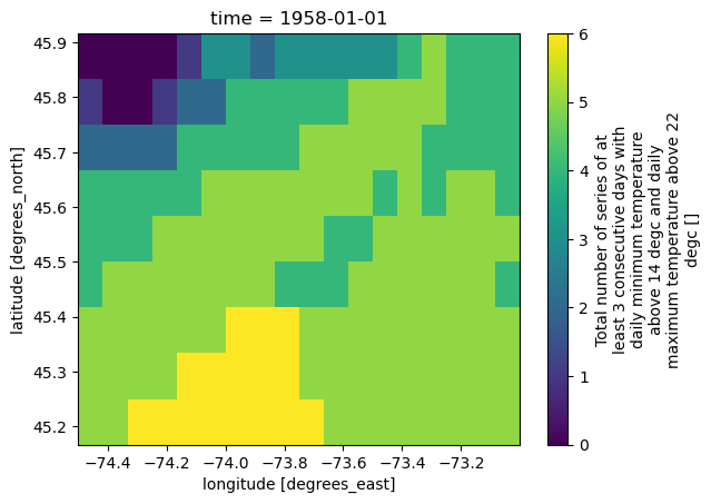
ds.heat_wave_frequency.plot()

<matplotlib.collections.QuadMesh at 0x7f7434053df0>

Streaming the data and showing on a map

The results are stored in a folder that is available to thredds, which provides a multiple services to access its datasets. In the case of large outputs, the user could view ths results of the analysis through an OPeNDAP service, so only the data to be shown is downloaded, and not the whole dataset.

Get the OPeNDAP url from the ‘wpsoutputs’

from urllib.parse import urlparse

output_url = result.get().output
print("output_url = ", output_url)
parsed = urlparse(output_url)
output_path = parsed.path.replace("wpsoutputs", "wps_outputs")
print("output_path = ", output_path)

output_thredds_url = (
    f"https://{parsed.hostname}/twitcher/ows/proxy/thredds/dodsC/birdhouse{output_path}"
)
print("output_thredds_url = ", output_thredds_url)

output_url =  https://pavics.ouranos.ca/wpsoutputs/finch/a745e506-cd09-11ef-af3f-0242ac130014/out.nc
output_path =  /wps_outputs/finch/a745e506-cd09-11ef-af3f-0242ac130014/out.nc
output_thredds_url =  https://pavics.ouranos.ca/twitcher/ows/proxy/thredds/dodsC/birdhouse/wps_outputs/finch/a745e506-cd09-11ef-af3f-0242ac130014/out.nc

This time, we will be using hvplot to build our figure. This tool is a part of the holoviz libraries and adds an easy interface to xarray datasets. Since geoviews and cartopy are also installed, we can simply pass geo=True and a choice for tiles to turn the plot into a map. If multiple times were present in the dataset, a slider would appear, letting the user choose the slice. As we are using an OPeNDAP link, only the data that needs to be plotted (the current time slice) is downloaded.

# NBVAL_IGNORE_OUTPUT
import hvplot.xarray

dsremote = xr.open_dataset(output_thredds_url)
dsremote.hvplot.quadmesh(
    "lon",
    "lat",
    "heat_wave_frequency",
    geo=True,
    alpha=0.8,
    frame_height=540,
    cmap="viridis",
    tiles="CartoLight",
)

---------------------------------------------------------------------------
ModuleNotFoundError                       Traceback (most recent call last)
Cell In[25], line 2
      1 # NBVAL_IGNORE_OUTPUT
----> 2 import hvplot.xarray
      4 dsremote = xr.open_dataset(output_thredds_url)
      5 dsremote.hvplot.quadmesh(
      6     "lon",
      7     "lat",
   (...)
     13     tiles="CartoLight",
     14 )

ModuleNotFoundError: No module named 'hvplot'