Working with the ECCC GeoAPI to access weather station data

Environment and Climate Change Canada (ECCC) hosts a data server compatible with the GeoAPI standard. This notebook shows how to send requests for daily climate station data and display the results.

Climate stations

The server holds different collections, and requests are made to a particular collection. Here we’ll start with the climate-station collection, which holds metadata about available stations, but no actual meteorological data. Useful queryables fields in this collection include DLY_FIRST_DATE and DLY_LAST_DATE, ENG_PROV_NAME, LATITUDE, LONGITUDE and ELEVATION and STATION_NAME, among many others.

Creating a request to the server for data

Let’s start by showing a map of all available stations locations in New-Brunswick. To do so, we first need to compose a URL request. The request includes the address of the server, the collection, then a query to filter results.

import os
from urllib.parse import urlencode, urljoin
from urllib.request import urlopen

os.environ["USE_PYGEOS"] = "0"  # force use Shapely with GeoPandas

import geopandas as gpd
import requests

# Compose the request
host = "https://api.weather.gc.ca/"
climate_stations = urljoin(host, "collections/climate-stations/items/")
query = {"ENG_PROV_NAME": "NEW-BRUNSWICK"}
url = f"{climate_stations}?{urlencode(query)}"
print(url)

# Send the request to the server
resp = requests.get(url)
resp

https://api.weather.gc.ca/collections/climate-stations/items/?ENG_PROV_NAME=NEW-BRUNSWICK

<Response [200]>

The response from the server is a Response class instance. What we’re interested in is the content of this response, which in this case is a geoJSON file.

# NBVAL_IGNORE_OUTPUT

resp.content[:300]

b'{"type":"FeatureCollection","features":[{"type":"Feature","properties":{"STN_ID":6288,"STATION_NAME":"ABERCROMBIE POINT","PROV_STATE_TERR_CODE":"NS","ENG_PROV_NAME":"NOVA SCOTIA","FRE_PROV_NAME":"NOUVELLE-\\u00c9COSSE","COUNTRY":"CAN","LATITUDE":453900000,"LONGITUDE":-624300000,"TIMEZONE":"AST","ELEV'

We’ll open the geoJSON using geopandas. We have a few options to do this:

• Load the response’ content using json.load, then create GeoDataFrame using the from_features class method;

• Save the response content to a file on disk, then open using geopandas.read_file;

• Save the response in an in-memory file using StringIO;

• Call geopandas.read_file(url) to let geopandas handle the data download.

Here we’ll use the last option, as it’s the simplest. Note that the first method ignores the feature id, which seems to create problems with visualization with folium below.

# NBVAL_IGNORE_OUTPUT

# The first approach would look like this:
# import json
# stations = gpd.GeoDataFrame.from_features(json.loads(resp.content))

# The second approach would look like this:
with urlopen(url=str(url)) as req:
    stations = gpd.read_file(filename=req, engine="fiona")
stations.head()

	id	STN_ID	STATION_NAME	PROV_STATE_TERR_CODE	ENG_PROV_NAME	FRE_PROV_NAME	COUNTRY	LATITUDE	LONGITUDE	TIMEZONE	...	HLY_FIRST_DATE	HLY_LAST_DATE	DLY_FIRST_DATE	DLY_LAST_DATE	MLY_FIRST_DATE	MLY_LAST_DATE	HAS_MONTHLY_SUMMARY	HAS_NORMALS_DATA	HAS_HOURLY_DATA	geometry
0	8200015	6288	ABERCROMBIE POINT	NS	NOVA SCOTIA	NOUVELLE-ÉCOSSE	CAN	453900000	-624300000	AST	...	NaT	NaT	1973-09-01	1978-12-31	1973-01-01	1978-12-01	Y	N	N	POINT (-62.71667 45.65)
1	8200100	6289	ANNAPOLIS ROYAL	NS	NOVA SCOTIA	NOUVELLE-ÉCOSSE	CAN	444500000	-653100000	AST	...	NaT	NaT	1914-04-01	2007-06-04	1914-01-01	2006-02-01	Y	N	N	POINT (-65.51667 44.75)
2	8200150	6290	ANTIGONISH	NS	NOVA SCOTIA	NOUVELLE-ÉCOSSE	CAN	453800000	-615800000	AST	...	NaT	NaT	1880-12-01	1947-12-31	1880-01-01	1947-12-01	Y	N	N	POINT (-61.96667 45.63333)
3	8200151	6291	ANTIGONISH	NS	NOVA SCOTIA	NOUVELLE-ÉCOSSE	CAN	453700000	-615900000	AST	...	NaT	NaT	1979-07-01	1982-12-31	1979-01-01	1982-12-01	Y	N	N	POINT (-61.98333 45.61667)
4	8200155	6292	APRIL BROOK IHD	NS	NOVA SCOTIA	NOUVELLE-ÉCOSSE	CAN	461400000	-610800000	AST	...	NaT	NaT	1966-12-01	1976-01-31	1966-01-01	1976-12-01	Y	N	N	POINT (-61.13333 46.23333)

5 rows × 34 columns

Filter stations

Now let’s say we want to filter the stations that were in operations for at least 50 years. What we’ll do is create a new column n_days and filter on it.

# NBVAL_IGNORE_OUTPUT

import pandas as pd

# Create a datetime.Timedelta object from the subtraction of two dates.
delta = pd.to_datetime(stations["DLY_LAST_DATE"]) - pd.to_datetime(
    stations["DLY_FIRST_DATE"]
)

# Get the number of days in the time delta
stations["n_days"] = delta.apply(lambda x: x.days)

# Compute condition
over_50 = stations["n_days"] > 50 * 365.25

# Index the data frame using the condition
select = stations[over_50]
select.head()

	id	STN_ID	STATION_NAME	PROV_STATE_TERR_CODE	ENG_PROV_NAME	FRE_PROV_NAME	COUNTRY	LATITUDE	LONGITUDE	TIMEZONE	...	HLY_LAST_DATE	DLY_FIRST_DATE	DLY_LAST_DATE	MLY_FIRST_DATE	MLY_LAST_DATE	HAS_MONTHLY_SUMMARY	HAS_NORMALS_DATA	HAS_HOURLY_DATA	geometry	n_days
1	8200100	6289	ANNAPOLIS ROYAL	NS	NOVA SCOTIA	NOUVELLE-ÉCOSSE	CAN	444500000	-653100000	AST	...	NaT	1914-04-01	2007-06-04	1914-01-01	2006-02-01	Y	N	N	POINT (-65.51667 44.75)	34032
2	8200150	6290	ANTIGONISH	NS	NOVA SCOTIA	NOUVELLE-ÉCOSSE	CAN	453800000	-615800000	AST	...	NaT	1880-12-01	1947-12-31	1880-01-01	1947-12-01	Y	N	N	POINT (-61.96667 45.63333)	24500
6	8200200	6294	AVON	NS	NOVA SCOTIA	NOUVELLE-ÉCOSSE	CAN	445300000	-641300000	AST	...	NaT	1949-11-01	2001-01-31	1949-01-01	2001-01-01	Y	N	N	POINT (-64.21667 44.88333)	18719
9	8200300	6297	BADDECK	NS	NOVA SCOTIA	NOUVELLE-ÉCOSSE	CAN	460600000	-604500000	AST	...	NaT	1875-06-01	2000-01-31	1875-01-01	2000-01-01	Y	N	N	POINT (-60.75 46.1)	45534
12	8200500	6300	BEAR RIVER	NS	NOVA SCOTIA	NOUVELLE-ÉCOSSE	CAN	443400000	-653800000	AST	...	NaT	1952-11-01	2006-02-28	1952-01-01	2006-02-01	Y	Y	N	POINT (-65.63333 44.56667)	19477

5 rows × 35 columns

Map the data

We can then simply map the locations of station with at least 50 years of data using the explore method. This will display an interactive base map and overlay the station locations, where on a station marker will display this station’s information.

On top of this map, we’ll add controls to draw a rectangle. To use the drawing tool, click on the square on the left hand side menu, and the click and drag to draw a rectangle over the area of interest. Once that’s done, click on the Export button on the right of the map. This will download a file called data.geojson

from folium.plugins import Draw

# Add control to draw a rectangle, and an export button.
draw_control = Draw(
    draw_options={
        "polyline": False,
        "poly": False,
        "circle": False,
        "polygon": False,
        "marker": False,
        "circlemarker": False,
        "rectangle": True,
    },
    export=True,
)

# The map library Folium chokes on columns including time stamps, so we first select the data to plot.
m = select[["geometry", "n_days"]].explore("n_days")
draw_control.add_to(m)
m

Make this Notebook Trusted to load map: File -> Trust Notebook

Filter stations using bounding box

Next, we’ll use the bounding box drawn on the map to select a subset of stations. We first open the data.geojson file downloaded to disk, create a shapely object and use it filter stations.

# NBVAL_IGNORE_OUTPUT

# Adjust directory if running this locally.
# rect = gpd.read_file("~/Downloads/data.geojson")

# Here we're using an existing file so the notebook runs without user interaction.
rect = gpd.read_file(filename="./data.geojson", engine="fiona")

# Filter stations DataFrame using bbox
inbox = select.within(rect.loc[0].geometry)

print("Number of stations within sub-region: ", sum(inbox))
sub_select = select[inbox]
sub_select.head()

Number of stations within sub-region:  9

	id	STN_ID	STATION_NAME	PROV_STATE_TERR_CODE	ENG_PROV_NAME	FRE_PROV_NAME	COUNTRY	LATITUDE	LONGITUDE	TIMEZONE	...	HLY_LAST_DATE	DLY_FIRST_DATE	DLY_LAST_DATE	MLY_FIRST_DATE	MLY_LAST_DATE	HAS_MONTHLY_SUMMARY	HAS_NORMALS_DATA	HAS_HOURLY_DATA	geometry	n_days
2	8200150	6290	ANTIGONISH	NS	NOVA SCOTIA	NOUVELLE-ÉCOSSE	CAN	453800000	-615800000	AST	...	NaT	1880-12-01	1947-12-31	1880-01-01	1947-12-01	Y	N	N	POINT (-61.96667 45.63333)	24500
9	8200300	6297	BADDECK	NS	NOVA SCOTIA	NOUVELLE-ÉCOSSE	CAN	460600000	-604500000	AST	...	NaT	1875-06-01	2000-01-31	1875-01-01	2000-01-01	Y	N	N	POINT (-60.75 46.1)	45534
41	8201000	6329	COLLEGEVILLE	NS	NOVA SCOTIA	NOUVELLE-ÉCOSSE	CAN	452900000	-620100000	AST	...	NaT	1916-06-01	2016-09-30	1916-01-01	2006-02-01	Y	Y	N	POINT (-62.01667 45.48333)	36646
48	8201410	6336	DEMING	NS	NOVA SCOTIA	NOUVELLE-ÉCOSSE	CAN	451259007	-611040090	AST	...	NaT	1956-10-01	2011-12-31	1956-01-01	2006-02-01	Y	Y	N	POINT (-61.1778 45.21639)	20179
153	8204480	6441	PORT HASTINGS	NS	NOVA SCOTIA	NOUVELLE-ÉCOSSE	CAN	453800000	-612400000	AST	...	NaT	1874-01-01	1989-09-30	1874-01-01	1989-12-01	Y	N	N	POINT (-61.4 45.63333)	42275

5 rows × 35 columns

Request meteorological data

Now we’ll make a request for actual meteorological data from the stations filtered above. For this, we’ll use the Daily Climate Observations collection (climate-daily). Here, we’re picking just one station but we could easily loop on each station.

# NBVAL_IGNORE_OUTPUT

coll = urljoin(host, "collections/climate-daily/items/")
station_id = "8201410"

# Restricting the number of entries returned to keep things fast.
queries = {"CLIMATE_IDENTIFIER": station_id, "limit": 365}
url = f"{coll}?{urlencode(queries)}"

print("Request: ", url)
with urlopen(url=str(url)) as req:
    data = gpd.read_file(filename=req, engine="fiona")
data.head()

Request:  https://api.weather.gc.ca/collections/climate-daily/items/?CLIMATE_IDENTIFIER=8201410&limit=365

	id	TOTAL_PRECIPITATION_FLAG	MAX_TEMPERATURE_FLAG	MAX_TEMPERATURE	LOCAL_MONTH	MIN_TEMPERATURE	PROVINCE_CODE	CLIMATE_IDENTIFIER	STATION_NAME	MAX_REL_HUMIDITY	...	MEAN_TEMPERATURE	MEAN_TEMPERATURE_FLAG	TOTAL_PRECIPITATION	TOTAL_RAIN_FLAG	SNOW_ON_GROUND	COOLING_DEGREE_DAYS_FLAG	DIRECTION_MAX_GUST_FLAG	TOTAL_SNOW_FLAG	SNOW_ON_GROUND_FLAG	geometry
0	8201410.1996.6.13	None	None	12.5	6	9.0	NS	8201410	DEMING	None	...	10.8	None	0.0	None	0.0	None	None	None	None	POINT (-61.1778 45.21639)
1	8201410.1993.12.17	None	None	0.5	12	-2.5	NS	8201410	DEMING	None	...	-1.0	None	0.0	None	0.0	None	None	None	None	POINT (-61.1778 45.21639)
2	8201410.1967.11.6	None	None	8.9	11	3.9	NS	8201410	DEMING	None	...	6.4	None	0.0	None	0.0	None	None	None	None	POINT (-61.1778 45.21639)
3	8201410.2003.1.14	None	None	-3.5	1	-6.0	NS	8201410	DEMING	None	...	-4.8	None	0.0	None	45.0	None	None	None	None	POINT (-61.1778 45.21639)
4	8201410.2009.1.30	None	None	-1.0	1	-5.5	NS	8201410	DEMING	None	...	-3.3	None	0.0	None	5.0	None	None	None	None	POINT (-61.1778 45.21639)

5 rows × 36 columns

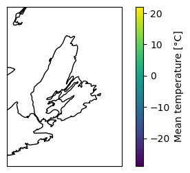
We can also send a request for data inside a bounding box at a specific date.

bbox = rect.iloc[0].geometry.bounds
print("Bounding box: ", bbox)
queries = {
    "bbox": str(bbox).strip("()"),
    "LOCAL_DATE": "2000-01-01 00:00:00",
    "limit": 100,
}
url = f"{coll}?{urlencode(queries)}"

with urlopen(url=str(url)) as req:
    snapshot = gpd.read_file(filename=req, engine="fiona")

Bounding box:  (-62.186675, 44.78125, -59.123882, 47.53125)

from cartopy import crs as ccrs
from matplotlib import pyplot as plt

# Create map projection
proj = ccrs.PlateCarree()

# If using another projection, remember you'll need to reproject the snapshot's coordinates.
# snapshot.to_crs(proj, inplace=True)

# Create figure and axes
fig = plt.figure(figsize=(5, 3))
ax = fig.add_subplot(projection=proj)

# Set the map extent to the bounding box and draw the coastlines
ax.set_extent([bbox[0], bbox[2], bbox[1], bbox[3]])
ax.coastlines()

# Plot markers color-coded according to the temperature recorded.
ax = snapshot.plot(column="MEAN_TEMPERATURE", ax=ax, cmap=plt.cm.viridis, legend=True)

# Add a label to the colorbar
cax = ax.figure.axes[-1]
cax.set_ylabel("Mean temperature [°C]")

Text(448.07777777777784, 0.5, 'Mean temperature [°C]')

Another useful filter is on dates and times. Let’s say we only want data in a given period, we simply create a request with the datetime argument and a / separating the start and end dates. You may leave the start or end date open-ended using .. instead of a date time string.

query = {
    "CLIMATE_IDENTIFIER": station_id,
    "datetime": "1990-01-01 00:00:00/1991-01-01 00:00:00",
}
url = f"{coll}?{urlencode(query)}"

print(url)
with urlopen(url=str(url)) as req:
    gdf = gpd.read_file(filename=req, engine="fiona")

https://api.weather.gc.ca/collections/climate-daily/items/?CLIMATE_IDENTIFIER=8201410&datetime=1990-01-01+00%3A00%3A00%2F1991-01-01+00%3A00%3A00

# Convert the datetime string to a datetime object
gdf["LOCAL_DATE"] = pd.to_datetime(gdf["LOCAL_DATE"])

# Create a time series out of the column for mean temperature
ts = gdf.set_index("LOCAL_DATE")["MEAN_TEMPERATURE"]

# Plot the time series
ax = ts.plot()
ax.set_xlabel("Time")
ax.set_ylabel("Mean temperature [°C]")
ax.set_title(gdf.iloc[0]["STATION_NAME"])
plt.show()

Adjusted and Homogenized Canadian Climate Data (AHCCD)

The Adjusted and Homogenized Canadian Climate Data (AHCCD) datasets from ECCC are climate station data adjusted to account for discontinuities in the record, such as instrument relocation. The collections related to these datasets are ahccd-stations for station metadata, ahccd-annual, ahccd-monthly and ahccd-seasonal for temporally aggregated time series, and ahccd-trends for trends computed on the data.

Now, unfortunately, the fields for these datasets are different from those of the climate stations… One strategy to find out what keywords are accepted is to make a query with no filter except for limit=1. Another is to go to the collection search page (click on the link printed below), and inspect the column names.

# NBVAL_IGNORE_OUTPUT

# The url to query station metadata - this should behave similarly as `climate-stations`
ahccd_stations = urljoin(host, "collections/ahccd-stations/items/")
query = {"limit": 1}
url = f"{ahccd_stations}?{urlencode(query)}"

print(url)
with urlopen(url=str(url)) as req:
    display(gpd.read_file(filename=req, engine="fiona"))

https://api.weather.gc.ca/collections/ahccd-stations/items/?limit=1

	id	identifier__identifiant	station_id__id_station	station_name__nom_station	measurement_type__type_mesure	period__periode	trend_value__valeur_tendance	elevation__elevation	province__province	joined__rejoint	year_range__annees	start_date__date_debut	end_date__date_fin	geometry
0	2400305	2400305	2400305	ALERT	temp_mean	Ann	1.5	65	NU	1	1951-2020	1950-07-01	2020-12-01	POINT (-62.33 82.5)

So if we want to see the stations in Yukon, we’d have to query with the province__province keyword… Now how do you know what code to use for provinces? One solution is to go again to the collection search page, zoom on the area of interest and click on the check box to “Only show items by map view”, then inspect the results.

# NBVAL_IGNORE_OUTPUT

query = {"province__province": "YT"}
url = f"{ahccd_stations}?{urlencode(query)}"

print(url)
with urlopen(url=str(url)) as req:
    display(gpd.read_file(filename=req, engine="fiona"))

https://api.weather.gc.ca/collections/ahccd-stations/items/?province__province=YT

	id	identifier__identifiant	station_id__id_station	station_name__nom_station	measurement_type__type_mesure	period__periode	trend_value__valeur_tendance	elevation__elevation	province__province	joined__rejoint	year_range__annees	start_date__date_debut	end_date__date_fin	geometry
0	2100100	2100100	2100100	AISHIHIK A	pressure_sea_level	Ann	NaN	966.20	YT	0	None	1953-01-01	1966-09-01	POINT (-137.48 61.65)
1	2100160	2100160	2100160	BEAVER CREEK A	pressure_sea_level	Ann	NaN	649.00	YT	1	None	1968-12-01	2014-12-01	POINT (-140.87 62.41)
2	2100400	2100400	2100400	DAWSON	pressure_sea_level	Ann	NaN	320.00	YT	0	None	1953-01-01	1976-01-01	POINT (-139.43 64.05)
3	2100402	2100402	2100402	DAWSON A	pressure_sea_level	Ann	NaN	370.30	YT	1	None	1976-02-01	2014-12-01	POINT (-139.13 64.04)
4	2100517	2100517	2100517	FARO A	pressure_sea_level	Ann	NaN	716.60	YT	1	None	1987-10-01	2014-12-01	POINT (-133.38 62.21)
5	2100636	2100636	2100636	HERSCHEL ISLAND	pressure_sea_level	Ann	NaN	1.20	YT	0	None	1986-10-01	2014-12-01	POINT (-138.91 69.57)
6	2100685	2100685	2100685	KOMAKUK BEACH A	pressure_sea_level	Ann	NaN	7.30	YT	0	None	1973-08-01	1993-06-01	POINT (-140.18 69.58)
7	2100800	2100800	2100800	OLD CROW A	pressure_sea_level	Ann	NaN	251.20	YT	1	None	1975-08-01	2014-12-01	POINT (-139.84 67.57)
8	2100935	2100935	2100935	ROCK RIVER	pressure_sea_level	Ann	NaN	731.00	YT	0	None	1989-09-01	2014-12-01	POINT (-136.22 66.98)
9	2101000	2101000	2101000	SNAG A	pressure_sea_level	Ann	NaN	586.70	YT	0	None	1953-01-01	1966-08-01	POINT (-140.4 62.37)
10	2100300	2100300	2100300	CARMACKS	snow	Ann	NaN	525.00	YT	0	None	1964-01-01	2008-02-01	POINT (-136.3 62.1)
11	2100460	2100460	2100460	DRURY CREEK	snow	Ann	NaN	609.00	YT	0	None	1970-01-01	2009-04-01	POINT (-134.39 62.2019)
12	2100631	2100631	2100631	HAINES JUNCTION	snow	Ann	NaN	596.00	YT	1	None	1945-01-01	2008-09-01	POINT (-137.5053 60.7495)
13	2101081	2101081	2101081	SWIFT RIVER	snow	Ann	NaN	891.00	YT	0	None	1967-01-01	2008-02-01	POINT (-131.1833 60)
14	2100182	2100182	2100182	BURWASH A	wind_speed	Ann	NaN	806.20	YT	1	None	1966-10-01	2014-12-01	POINT (-139.05 61.3667)
15	2100700	2100700	2100700	MAYO A	wind_speed	Ann	0.00	503.80	YT	1	1953-2014	1953-01-01	2014-12-01	POINT (-135.8667 63.6167)
16	2101100	2101100	2101100	TESLIN A	wind_speed	Ann	NaN	705.00	YT	1	None	1953-01-01	2014-12-01	POINT (-132.7359 60.1741)
17	2101200	2101200	2101200	WATSON LAKE A	wind_speed	Ann	-0.72	687.35	YT	0	1953-2014	1953-01-01	2014-11-01	POINT (-128.8223 60.1165)
18	2101300	2101300	2101300	WHITEHORSE A	wind_speed	Ann	-0.25	706.20	YT	1	1953-2014	1953-01-01	2014-12-01	POINT (-135.0688 60.7095)
19	2100184	2100184	2100184	BURWASH	temp_mean	Ann	NaN	807.00	YT	1	None	1966-10-01	2020-12-01	POINT (-139.02 61.37)
20	2100301	2100301	2100301	CARMACKS	temp_mean	Ann	NaN	543.00	YT	1	None	1963-08-01	2020-12-01	POINT (-136.2 62.12)
21	2100LRP	2100LRP	2100LRP	DAWSON	temp_mean	Ann	2.29	370.00	YT	1	1901-2020	1901-01-01	2020-12-01	POINT (-139.13 64.07)
22	2100518	2100518	2100518	FARO_(AUT)	temp_mean	Ann	NaN	717.00	YT	1	None	1977-12-01	2020-12-01	POINT (-133.38 62.2)
23	2100630	2100630	2100630	HAINES_JUNCTION	temp_mean	Ann	NaN	595.00	YT	0	None	1944-10-01	2020-12-01	POINT (-137.58 60.77)
24	2100660	2100660	2100660	IVVAVIK_NAT_PARK	temp_mean	Ann	NaN	244.00	YT	0	None	1995-07-01	2020-12-01	POINT (-140.15 69.17)
25	2100682	2100682	2100682	KOMAKUK_BEACH	temp_mean	Ann	NaN	13.00	YT	1	None	1958-07-01	2018-06-01	POINT (-140.2 69.62)
26	2100693	2100693	2100693	MACMILLAN_PASS	temp_mean	Ann	NaN	1379.00	YT	0	None	1998-02-01	2020-12-01	POINT (-130.03 63.25)
27	2100701	2100701	2100701	MAYO	temp_mean	Ann	NaN	504.00	YT	1	None	1924-10-01	2020-12-01	POINT (-135.87 63.62)
28	2100805	2100805	2100805	OLD_CROW	temp_mean	Ann	NaN	251.00	YT	1	None	1951-09-01	2020-12-01	POINT (-139.83 67.57)
29	2100880	2100880	2100880	PELLY_RANCH	temp_mean	Ann	NaN	445.00	YT	0	None	1955-01-01	2017-08-01	POINT (-137.32 62.83)
30	2100941	2100941	2100941	ROSS_RIVER	temp_mean	Ann	NaN	698.00	YT	1	None	1961-12-01	2008-08-01	POINT (-132.45 61.98)
31	2100950	2100950	2100950	SHINGLE_POINT	temp_mean	Ann	NaN	49.00	YT	0	None	1957-06-01	2020-12-01	POINT (-137.22 68.95)
32	2101102	2101102	2101102	TESLIN	temp_mean	Ann	NaN	705.00	YT	1	None	1943-10-01	2020-12-01	POINT (-132.73 60.17)
33	2101135	2101135	2101135	TUCHITUA	temp_mean	Ann	NaN	724.00	YT	0	None	1967-01-01	2014-09-01	POINT (-129.22 60.93)
34	2101204	2101204	2101204	WATSON_LAKE	temp_mean	Ann	1.50	683.00	YT	1	1939-2020	1938-10-01	2020-12-01	POINT (-128.83 60.12)
35	2101310	2101310	2101310	WHITEHORSE	temp_mean	Ann	NaN	707.00	YT	1	None	1959-02-01	2020-12-01	POINT (-135.1 60.73)
36	2101303	2101303	2101303	WHITEHORSE_A	temp_mean	Ann	1.70	706.00	YT	1	1943-2020	1942-04-01	2020-12-01	POINT (-135.07 60.72)

Let’s pick the Dawson station (2100LRP), which seems to have a long record. Again, use the trick above to see which fields are accepted.

# NBVAL_IGNORE_OUTPUT

ahccd_mon = urljoin(host, "collections/ahccd-monthly/items/")
query = {"station_id__id_station": "2100LRP"}
url = f"{ahccd_mon}?{urlencode(query)}"

print(url)
with urlopen(url=str(url)) as req:
    mts = gpd.read_file(filename=req, engine="fiona")
mts.head()

https://api.weather.gc.ca/collections/ahccd-monthly/items/?station_id__id_station=2100LRP

	id	wind_speed__vitesse_vent	period_group__groupe_periode	wind_speed_units__vitesse_vent_unites	lon__long	rain__pluie	snow__neige	date	temp_mean__temp_moyenne	identifier__identifiant	...	lat__lat	temp_max_units__temp_max_unites	temp_min__temp_min	station_id__id_station	rain_units__pluie_unites	pressure_sea_level__pression_niveau_mer	pressure_station__pression_station	temp_mean_units__temp_moyenne_unites	total_precip_units__precip_totale_unites	geometry
0	2100LRP.1983.03	None	Monthly	kph	-139.13	None	None	1983-03	-15.7	2100LRP.1983.03	...	64.07	C	-24.5	2100LRP	mm	None	None	C	mm	POINT (-139.13 64.07)
1	2100LRP.1921.03	None	Monthly	kph	-139.13	None	None	1921-03	-16.8	2100LRP.1921.03	...	64.07	C	-24.7	2100LRP	mm	None	None	C	mm	POINT (-139.13 64.07)
2	2100LRP.1992.06	None	Monthly	kph	-139.13	None	None	1992-06	14.2	2100LRP.1992.06	...	64.07	C	6.4	2100LRP	mm	None	None	C	mm	POINT (-139.13 64.07)
3	2100LRP.1938.03	None	Monthly	kph	-139.13	None	None	1938-03	-13.7	2100LRP.1938.03	...	64.07	C	-22.9	2100LRP	mm	None	None	C	mm	POINT (-139.13 64.07)
4	2100LRP.1963.09	None	Monthly	kph	-139.13	None	None	1963-09	6.5	2100LRP.1963.09	...	64.07	C	0.9	2100LRP	mm	None	None	C	mm	POINT (-139.13 64.07)

5 rows × 28 columns

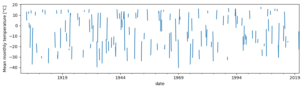
Now let’s plot the mean temperature time series. Note that the server does not necessarily return a continuous time series, and when plotting time series with gaps, matplotlib just draws a continuous line between values. To convey the presence of missing values, here we’ll use the asfreq("MS") method to fill-in gaps in the time series with explicit missing values.

# Set the DataFrame index to a datetime object and sort it
mts.set_index(pd.to_datetime(mts["date"]), inplace=True)
mts.sort_index(inplace=True)

# Convert the temperature to a continuous monthly time series (so missing values are visible in the graphic)
tas = mts["temp_mean__temp_moyenne"].asfreq("MS")

# Mask missing values
tas.mask(tas < -300, inplace=True)

tas.plot(figsize=(12, 3))
plt.ylabel("Mean monthly temperature [°C]")

Text(0, 0.5, 'Mean monthly temperature [°C]')