Working with the ClimEx Large Ensemble
Analyzing ClimEx
ClimEx is a project investigating the influence of climate change on hydro-meteorological extremes. To understand the effect of natural variability on the occurrence of rare extreme events, ClimEx ran 50 independent simulations, increasing the sample size available.
Analyzing simulation outputs from large ensembles can get tedious due to the large number of individual netCDF files to handle. To simplify data access, we’ve created an aggregated view of daily precipitation and temperature for all 50 ClimEx realizations from 1955 to 2100.
The first step is to open the dataset, whose path can be found in the climex catalog. Although there are currently 36 250 individual netCDF files, there is only one link in the catalogue.
import logging
import warnings

import intake
import numba
import xarray as xr
import xclim
from clisops.core.subset import subset_gridpoint
from dask.diagnostics import ProgressBar
from dask.distributed import Client
from IPython.display import HTML, clear_output

warnings.simplefilter("ignore", category=UserWarning)

from xclim import ensembles as xens

warnings.simplefilter("ignore", category=numba.core.errors.NumbaDeprecationWarning)

# fmt: off
climex = "https://pavics.ouranos.ca/catalog/climex.json"  # TEST_USE_PROD_DATA
cat = intake.open_esm_datastore(climex)
# fmt: on

cat.df.head()
| license_type | title | institution | driving_model_id | driving_experiment | type | processing | project_id | frequency | modeling_realm | variable_name | variable_long_name | path | |
|---|---|---|---|---|---|---|---|---|---|---|---|---|---|
| 0 | permissive non-commercial | The ClimEx CRCM5 Large Ensemble | Ouranos Consortium on Regional Climatology and... | CCCma-CanESM2 | historical, rcp85 | RCM | raw | CLIMEX | day | atmos | ['tasmin', 'tasmax', 'tas', 'pr', 'prsn', 'rot... | ['Daily Minimum Near-Surface Temperature minim... | https://pavics.ouranos.ca/twitcher/ows/proxy/t... |
# Opening the link takes a while because the server creates an aggregated view of 435,000 individual files.
url = cat.df.path[0]
ds = xr.open_dataset(url, chunks=dict(realization=2, time=30 * 3), engine="netcdf4")
ds
<xarray.Dataset> Size: 6TB
Dimensions:       (time: 52924, realization: 50, rlat: 280, rlon: 280)
Coordinates:
  * time          (time) object 423kB 1955-01-01 00:00:00 ... 2099-12-30 00:0...
  * realization   (realization) |S64 3kB b'historical-r1-r10i1p1' ... b'histo...
  * rlat          (rlat) float64 2kB -12.61 -12.51 -12.39 ... 17.85 17.96 18.07
  * rlon          (rlon) float64 2kB 2.695 2.805 2.915 ... 33.17 33.28 33.39
    lat           (rlat, rlon) float32 314kB dask.array<chunksize=(280, 280), meta=np.ndarray>
    lon           (rlat, rlon) float32 314kB dask.array<chunksize=(280, 280), meta=np.ndarray>
Data variables:
    rotated_pole  (time) |S64 3MB dask.array<chunksize=(90,), meta=np.ndarray>
    plev          float64 8B ...
    tasmin        (realization, time, rlat, rlon) float32 830GB dask.array<chunksize=(2, 90, 280, 280), meta=np.ndarray>
    tasmax        (realization, time, rlat, rlon) float32 830GB dask.array<chunksize=(2, 90, 280, 280), meta=np.ndarray>
    tas           (realization, time, rlat, rlon) float32 830GB dask.array<chunksize=(2, 90, 280, 280), meta=np.ndarray>
    pr            (realization, time, rlat, rlon) float32 830GB dask.array<chunksize=(2, 90, 280, 280), meta=np.ndarray>
    prsn          (realization, time, rlat, rlon) float32 830GB dask.array<chunksize=(2, 90, 280, 280), meta=np.ndarray>
    prw           (realization, time, rlat, rlon) float32 830GB dask.array<chunksize=(2, 90, 280, 280), meta=np.ndarray>
    clwvi         (realization, time, rlat, rlon) float32 830GB dask.array<chunksize=(2, 90, 280, 280), meta=np.ndarray>
Attributes: (12/29)
    Conventions:           CF-1.6
    DODS.dimName:          string1
    DODS.strlen:           1
    EXTRA_DIMENSION.bnds:  2
    NCO:                   "4.5.2"
    abstract:              The ClimEx CRCM5 Large Ensemble of high-resolution...
    ...                    ...
    product:               output
    project_id:            CLIMEX
    rcm_version_id:        v3331
    terms_of_use:          http://www.climex-project.org/sites/default/files/...
    title:                 The ClimEx CRCM5 Large Ensemble
type: RCMThe CLIMEX dataset currently stores 5 daily variables, simulated by CRCM5 driven by CanESM2 using the representative concentration pathway RCP8.5:
pr: mean daily precipitation fluxprsn: mean daily snowfall fluxtas: mean daily temperaturetasmin: minimum daily temperaturetasmax: maximum daily temperature
The variables are stored along spatial dimensions (rotated latitude and longitude), time (1955-2100), and realizations (50 members). These members are created by first running five members from CanESM2 from 1850 to 1950, then small perturbations are applied in 1950 to spawn 10 members from each original member, to yield a total of 50 global realizations. Each realization is then dynamically downscaled to 12 km resolution over Québec.

ds.realization[:5].data.tolist()
[b'historical-r1-r10i1p1',
 b'historical-r1-r1i1p1',
 b'historical-r1-r2i1p1',
 b'historical-r1-r3i1p1',
 b'historical-r1-r4i1p1']
Creating maps of ClimEx fields
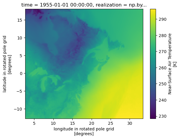
The data is on a rotated pole grid, and the actual geographic latitudes and longitudes of grid centroids are stored in the variables with the same name. We can plot the data directly using the native rlat and rlon coordinates easily.
# NBVAL_IGNORE_OUTPUT
from matplotlib import pyplot as plt

with ProgressBar():
    field = ds.tas.isel(time=0, realization=0).load()
    field.plot()
[ ] | 0% Completed | 522.75 us
[ ] | 0% Completed | 101.73 ms
[ ] | 0% Completed | 202.99 ms
[ ] | 0% Completed | 304.75 ms
[ ] | 0% Completed | 406.44 ms
[ ] | 0% Completed | 507.73 ms
[ ] | 0% Completed | 608.64 ms
[ ] | 0% Completed | 709.47 ms
[ ] | 0% Completed | 810.25 ms
[ ] | 0% Completed | 911.58 ms
[ ] | 0% Completed | 1.01 s
[ ] | 0% Completed | 1.12 s
[ ] | 0% Completed | 1.22 s
[ ] | 0% Completed | 1.32 s
[ ] | 0% Completed | 1.42 s
[ ] | 0% Completed | 1.52 s
[ ] | 0% Completed | 1.62 s
[########################## ] | 66% Completed | 1.72 s
[########################## ] | 66% Completed | 1.82 s
[########################## ] | 66% Completed | 1.93 s
[########################## ] | 66% Completed | 2.03 s
[########################## ] | 66% Completed | 2.13 s
[########################## ] | 66% Completed | 2.23 s
[########################## ] | 66% Completed | 2.33 s
[########################## ] | 66% Completed | 2.43 s
[########################## ] | 66% Completed | 2.53 s
[########################## ] | 66% Completed | 2.64 s
[########################## ] | 66% Completed | 2.74 s
[########################## ] | 66% Completed | 2.84 s
[########################## ] | 66% Completed | 2.94 s
[########################## ] | 66% Completed | 3.04 s
[########################## ] | 66% Completed | 3.15 s
[########################## ] | 66% Completed | 3.25 s
[########################## ] | 66% Completed | 3.35 s
[########################## ] | 66% Completed | 3.45 s
[########################## ] | 66% Completed | 3.55 s
[########################## ] | 66% Completed | 3.65 s
[########################## ] | 66% Completed | 3.75 s
[########################## ] | 66% Completed | 3.85 s
[########################## ] | 66% Completed | 3.96 s
[########################## ] | 66% Completed | 4.06 s
[########################## ] | 66% Completed | 4.16 s
[########################## ] | 66% Completed | 4.26 s
[########################## ] | 66% Completed | 4.36 s
[########################## ] | 66% Completed | 4.46 s
[########################## ] | 66% Completed | 4.56 s
[########################## ] | 66% Completed | 4.67 s
[########################## ] | 66% Completed | 4.77 s
[########################## ] | 66% Completed | 4.87 s
[########################## ] | 66% Completed | 4.97 s
[########################## ] | 66% Completed | 5.07 s
[########################## ] | 66% Completed | 5.17 s
[########################## ] | 66% Completed | 5.27 s
[########################## ] | 66% Completed | 5.37 s
[########################## ] | 66% Completed | 5.48 s
[########################## ] | 66% Completed | 5.58 s
[########################## ] | 66% Completed | 5.68 s
[########################## ] | 66% Completed | 5.78 s
[########################################] | 100% Completed | 5.88 s
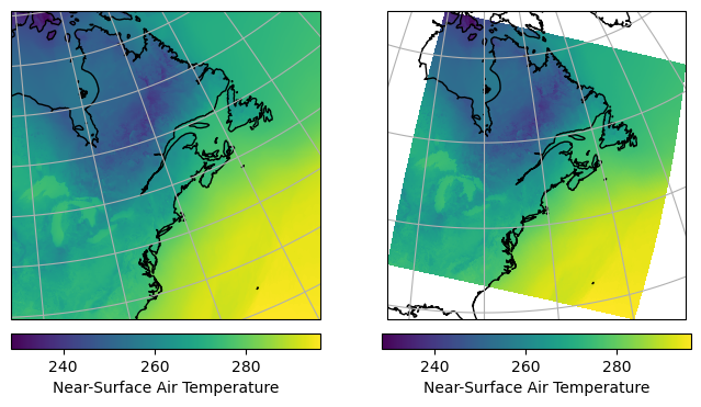
However, the axes are defined with respect to the rotated coordinates. To create a map with correct geographic coordinates, we could use the real longitudes and latitudes (plt.pcolormesh(ds.lon, ds.lat, field)), but a better option is to create axes with the same projection used by the model. That is, we set the map projection to RotatedPole, using the coordinate reference system defined in the rotated_pole variable. We can use a similar approach to project the model output on another projection.
# NBVAL_IGNORE_OUTPUT
import cartopy.crs as ccrs

with ProgressBar():
    # The CRS for the rotated pole (data)
    rotp = ccrs.RotatedPole(
        pole_longitude=ds.rotated_pole.grid_north_pole_longitude,
        pole_latitude=ds.rotated_pole.grid_north_pole_latitude,
    )

    # The CRS for your map projection (can be anything)
    ortho = ccrs.Orthographic(central_longitude=-80, central_latitude=45)

    fig = plt.figure(figsize=(8, 4))

    # Plot data on the rotated pole projection directly
    ax = plt.subplot(1, 2, 1, projection=rotp)
    ax.coastlines()
    ax.gridlines()
    m = ax.pcolormesh(ds.rlon, ds.rlat, field)
    plt.colorbar(
        m, orientation="horizontal", label=field.long_name, fraction=0.046, pad=0.04
    )

    # Plot data on another projection, transforming it using the rotp crs.
    ax = plt.subplot(1, 2, 2, projection=ortho)
    ax.coastlines()
    ax.gridlines()
    m = ax.pcolormesh(
        ds.rlon, ds.rlat, field, transform=rotp
    )  # Note the transform parameter
    plt.colorbar(
        m, orientation="horizontal", label=field.long_name, fraction=0.046, pad=0.04
    )

    plt.show()
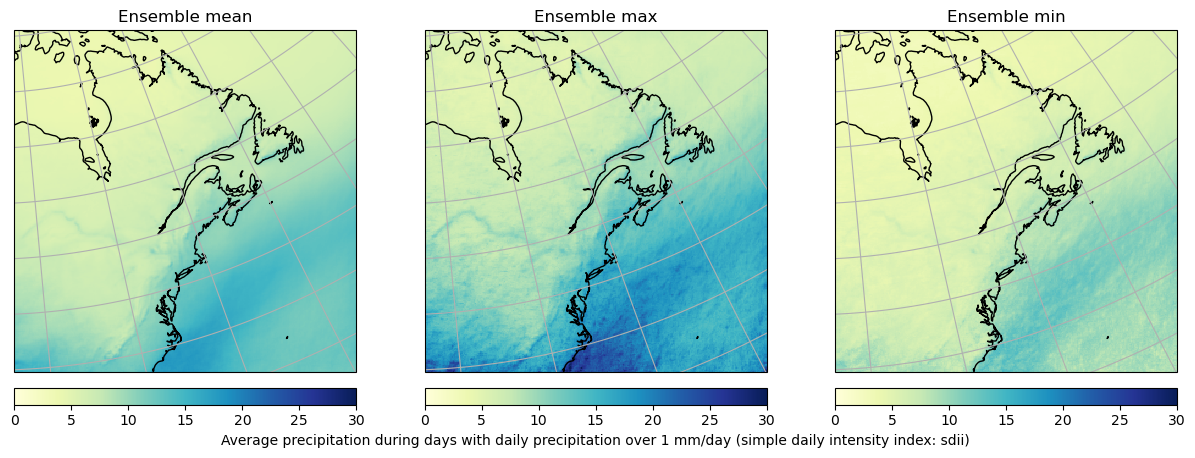
Computing climate indicators for ClimEx
Next we’ll compute a climate indicator as an example. We’ll compute the mean precipitation intensity for 50 members for the year 2000, then compute ensemble statistics between realizations. The amount of data that we’ll be requesting is, however, too big to go over the network in one request. To work around this, we need to first chunk the data in smaller dask.array portions by setting the chunks parameter when creating our dataset.
When selecting
xarraychunk sizes it is important to consider both the “on-disk” chunk sizes of the netcdf data and the type of calculation you are performing. For example, the Climex data variables_ChunkSizesattributes indicate on-disk chunk size for dimstime, rlat, rlonof[365 50 50]1. Using multiples of these values is a reasonable way to ensure that in-memorydaskchunks line up with the way that the data is stored on disk.The next step is to think about the calculation we wish to perform. In this case we wish to analyze a single year of data for all realizations over the entire spatial domain. Using something like
chunks = dict(realization=1, time=365, rlat=50*3, rlon=50*3)seems reasonable as a start. The general goal is to find a balance between chunk-size and a number of chunks … too many small chunks to process will create a lot of overhead and slow the calculation down. Huge chunks will use a lot of system memory causing other issues or data timeouts from the PAVICS thredds server. In this specific case having a largetimechunk could result in reading more data than necessary seeing as we are only interested in a single year.Enabling chunking also has the effect of making further computations on these chunks lazy. The next cell is thus going to execute almost instantly, because no data is transferred, and no computation executed. Calculations are launched when the data is actually needed, as when plotting graphics, saving to file, or when requested explicitly by calling the
compute,persist, orloadmethods. Below we make use of adask.distributedClient of worker processes to parallelize computations and improve performance.
1 In this case the `realization` chunk size is not included in the netcdf file attributes as this is a virtual dimension resulting from the NcML aggregation.
ds = xr.open_dataset(
    url, chunks=dict(realization=1, time=365, rlat=50 * 3, rlon=50 * 3)
)
xclim.set_options(check_missing="pct", missing_options={"pct": {"tolerance": 0.05}})
sdii = xclim.atmos.daily_pr_intensity(pr=ds.pr.sel(time="2000"))
sdii
<xarray.DataArray 'sdii' (realization: 50, time: 1, rlat: 280, rlon: 280)> Size: 31MB
dask.array<where, shape=(50, 1, 280, 280), dtype=float64, chunksize=(1, 1, 150, 150), chunktype=numpy.ndarray>
Coordinates:
  * realization  (realization) |S64 3kB b'historical-r1-r10i1p1' ... b'histor...
  * time         (time) object 8B 2000-01-01 00:00:00
  * rlat         (rlat) float64 2kB -12.61 -12.51 -12.39 ... 17.85 17.96 18.07
  * rlon         (rlon) float64 2kB 2.695 2.805 2.915 ... 33.17 33.28 33.39
    lat          (rlat, rlon) float32 314kB dask.array<chunksize=(150, 150), meta=np.ndarray>
    lon          (rlat, rlon) float32 314kB dask.array<chunksize=(150, 150), meta=np.ndarray>
Attributes:
    units:          mm d-1
    cell_methods:   time: mean
    history:        [2026-03-27 14:50:42] sdii: SDII(pr=pr, thresh='1 mm/day'...
    standard_name:  lwe_thickness_of_precipitation_amount
    long_name:      Average precipitation during days with daily precipitatio...
description: Annual simple daily intensity index (sdii) or annual aver...# NBVAL_IGNORE_OUTPUT
# Create a local client with 6 worker processes.
dask_kwargs = dict(
n_workers=6,
threads_per_worker=6,
memory_limit="4GB",
local_directory="/notebook_dir/writable-workspace/tmp",
silence_logs=logging.ERROR,
)
with Client(**dask_kwargs) as client:
clear_output()
display(
HTML(
f'<div class="alert alert-info"> Consult the client <a href="{client.dashboard_link}" target="_blank"><strong><em><u>Dashboard</u></em></strong></a> or the <strong><em>Dask jupyter sidebar</em></strong> to follow progress ... </div>'
)
)
out = xens.ensemble_mean_std_max_min(sdii.to_dataset())
out = out.load()
clear_output()
fig = plt.figure(figsize=(15, 5))
for ii, vv in enumerate([v for v in out.data_vars if "stdev" not in v]):
    ax = plt.subplot(1, 3, ii + 1, projection=rotp)

    ax.coastlines()
    ax.gridlines()
    m = ax.pcolormesh(
        out.rlon, out.rlat, out[vv].isel(time=0), vmin=0, vmax=30, cmap="YlGnBu"
    )
    c = plt.colorbar(
        m, orientation="horizontal", label=out[vv].long_name, fraction=0.046, pad=0.04
    )
    ax.set_title(f"Ensemble {vv.split('_')[-1]}")
    if ii != 1:
        c.set_label("")
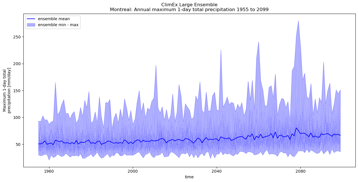
In the next example, we extract one grid point over Montréal to calculate the annual maximum 1-day precipitation for all years and ensemble members. In this case we would likely benefit by rethinking out chunk sizes.
Since we are only interested in a single grid-cell, there is no real need to have relatively large spatial chunks in the
rlonandrlatdimensions read into memory to simply be immediately discarded. In this case we reduce the spatial chunk size.Similarly, since we are only looking at a single point, we can likely get away with loading a large number of time steps into a single chunk.
# Subset over the Montréal gridpoint
ds = xr.open_dataset(url, chunks=dict(realization=1, time=365 * 50, rlon=25, rlat=25))
pt = subset_gridpoint(ds, lon=-73.69, lat=45.50)
print("Input dataset for Montreal :")
display(pt)
out = xclim.atmos.max_1day_precipitation_amount(pr=pt.pr, freq="YS")
print("Maximim 1-day precipitation `lazy` output ..")
out
Input dataset for Montreal :
<xarray.Dataset> Size: 78MB
Dimensions:       (time: 52924, realization: 50)
Coordinates:
  * time          (time) object 423kB 1955-01-01 00:00:00 ... 2099-12-30 00:0...
  * realization   (realization) |S64 3kB b'historical-r1-r10i1p1' ... b'histo...
    rlat          float64 8B 0.365
    rlon          float64 8B 16.12
    lat           float32 4B 45.45
    lon           float32 4B -73.7
Data variables:
    rotated_pole  (time) |S64 3MB dask.array<chunksize=(18250,), meta=np.ndarray>
    plev          float64 8B 0.0
    tasmin        (realization, time) float32 11MB dask.array<chunksize=(1, 18250), meta=np.ndarray>
    tasmax        (realization, time) float32 11MB dask.array<chunksize=(1, 18250), meta=np.ndarray>
    tas           (realization, time) float32 11MB dask.array<chunksize=(1, 18250), meta=np.ndarray>
    pr            (realization, time) float32 11MB dask.array<chunksize=(1, 18250), meta=np.ndarray>
    prsn          (realization, time) float32 11MB dask.array<chunksize=(1, 18250), meta=np.ndarray>
    prw           (realization, time) float32 11MB dask.array<chunksize=(1, 18250), meta=np.ndarray>
    clwvi         (realization, time) float32 11MB dask.array<chunksize=(1, 18250), meta=np.ndarray>
Attributes: (12/29)
    Conventions:           CF-1.6
    DODS.dimName:          string1
    DODS.strlen:           1
    EXTRA_DIMENSION.bnds:  2
    NCO:                   "4.5.2"
    abstract:              The ClimEx CRCM5 Large Ensemble of high-resolution...
    ...                    ...
    product:               output
    project_id:            CLIMEX
    rcm_version_id:        v3331
    terms_of_use:          http://www.climex-project.org/sites/default/files/...
    title:                 The ClimEx CRCM5 Large Ensemble
type: RCMMaximim 1-day precipitation `lazy` output ..
<xarray.DataArray 'rx1day' (realization: 50, time: 145)> Size: 29kB
dask.array<where, shape=(50, 145), dtype=float32, chunksize=(1, 50), chunktype=numpy.ndarray>
Coordinates:
  * realization  (realization) |S64 3kB b'historical-r1-r10i1p1' ... b'histor...
  * time         (time) object 1kB 1955-01-01 00:00:00 ... 2099-01-01 00:00:00
    rlat         float64 8B 0.365
    rlon         float64 8B 16.12
    lat          float32 4B 45.45
    lon          float32 4B -73.7
Attributes:
    units:          mm/day
    standard_name:  lwe_thickness_of_precipitation_amount
    cell_methods:   time: mean time: maximum over days
    history:        [2026-03-27 14:55:35] rx1day: RX1DAY(pr=pr, freq='YS') wi...
    long_name:      Maximum 1-day total precipitation
description: Annual maximum 1-day total precipitation# NBVAL_IGNORE_OUTPUT
# Compute the annual max 1-day precipitation
dask_kwargs = dict(
n_workers=6,
threads_per_worker=6,
memory_limit="4GB",
local_directory="/notebook_dir/writable-workspace/tmp",
silence_logs=logging.ERROR,
)
with Client(**dask_kwargs) as client:
# dashboard available at client.dashboard_link
clear_output()
display(
HTML(
f'<div class="alert alert-info"> Consult the client <a href="{client.dashboard_link}" target="_blank"><strong><em><u>Dashboard</u></em></strong></a> or the <strong><em>Dask jupyter sidebar</em></strong> to follow progress ... </div>'
)
)
out = out.load()
clear_output()
out_ens = xens.ensemble_mean_std_max_min(out.to_dataset())
fig = plt.figure(figsize=(15, 7))
ax = plt.subplot(1, 1, 1)
h1 = out.plot.line(ax=ax, x="time", color="b", linestyle=":", alpha=0.075, label=None)
h2 = plt.fill_between(
    x=out_ens.time.values,
    y1=out_ens.rx1day_max,
    y2=out_ens.rx1day_min,
    color="b",
    alpha=0.3,
    label="ensemble min - max",
)
h3 = plt.plot(
    out_ens.time.values, out_ens.rx1day_mean, color="b", label="ensemble mean"
)
handles, labels = ax.get_legend_handles_labels()
leg = ax.legend(handles[::-1], labels[::-1])
tit = plt.title(
    f"ClimEx Large Ensemble\nMontreal: {out.description} {out_ens.time.dt.year[0].values} to {out_ens.time.dt.year[-1].values}"
)