Web Coverage Service - Accessing GeoMet data using owslib
In this notebook we’ll connect to Environment Canada’s GeoMet service and fetch data using the WCS standard.
%matplotlib inline

from tempfile import NamedTemporaryFile

import matplotlib.pyplot as plt
import xarray as xr
from owslib.wcs import WebCoverageService
MSC GeoMet — GeoMet-Weather 2.38.0
['CAPS-Ocean_3km_MixedLayerThickness',
 'CAPS-Ocean_3km_SeaIceCompressiveStrength',
 'CAPS-Ocean_3km_SeaIceDivergence',
 'CAPS-Ocean_3km_SeaIceFraction',
 'CAPS-Ocean_3km_SeaIceInternalPressure',
 'CAPS-Ocean_3km_SeaIceShear',
 'CAPS-Ocean_3km_SeaIceSnowTemp',
 'CAPS-Ocean_3km_SeaIceSnowVolume',
 'CAPS-Ocean_3km_SeaIceVelocityX',
 'CAPS-Ocean_3km_SeaIceVelocityY']
Now let’s get some information about a given layer, here the mixed layer thickness.
layerid = "CAPS-Ocean_3km_MixedLayerThickness"
temp = wcs[layerid]
# Title
print("Layer title :", temp.title)
# bounding box
print("BoundingBox :", temp.boundingBoxWGS84)
# supported data formats - we'll use geotiff
print("Formats :", sorted(temp.supportedFormats))
# grid dimensions
print("Grid upper limits :", sorted(temp.grid.highlimits))
Layer title : None
BoundingBox : None
Formats : ['application/x-grib2', 'image/jpeg', 'image/netcdf', 'image/png', 'image/png; mode=8bit', 'image/tiff', 'image/vnd.jpeg-png', 'image/vnd.jpeg-png8', 'image/webp', 'image/x-aaigrid']
Grid upper limits : ['1829', '2229']
To request data, we need to call the getCoverage service, which requires us specifying the geographic projection, the bounding box, the resolution and format of the output. With GeoMet 2.0.1, we can now get layers in the netCDF format.
format_wcs = "image/netcdf"
bbox_wcs = temp.boundingboxes[0]["bbox"]  # Get the entire domain
crs_wcs = temp.boundingboxes[0]["nativeSrs"]  # Coordinate system
w = int(temp.grid.highlimits[0])
h = int(temp.grid.highlimits[1])

print("Format:", format_wcs)
print("Bounding box:", bbox_wcs)
print("Projection:", crs_wcs)
print(f"Resolution: {w} x {h}")

output = wcs.getCoverage(
    identifier=layerid,
    crs=crs_wcs,
    bbox=bbox_wcs,
    width=w,
    height=h,
    format=format_wcs,
)
Format: image/netcdf
Bounding box: (43.936456, -180.0, 90.0, 180.0)
Projection: http://www.opengis.net/def/crs/EPSG/0/4326
Resolution: 2229 x 1829
We then save the output to disk, open it normally using xarray and plot it’s variable.
# NBVAL_IGNORE_OUTPUT

tempfile = NamedTemporaryFile(prefix=layerid, suffix=".nc", delete=False)

with open(tempfile.name, "wb") as fh:
    fh.write(output.read())
tempfile.name
'/tmp/CAPS-Ocean_3km_MixedLayerThickness48i08jrm.nc'
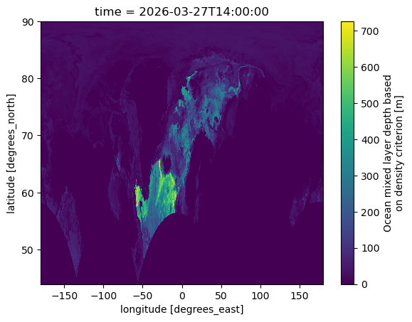
ds = xr.open_dataset(tempfile.name, engine="netcdf4")
print(ds.data_vars)
ds.sokaraml.plot()
plt.show()

# Clean up
tempfile.close()
Data variables:
    crs       |S1 1B ...
    sokaraml  (time, lat, lon) float32 16MB ...