Accessing and analysing Canadian Surface Reanalysis (CaSR) data in the PAVICS JupyterLab¶

This notebook demonstrates how to access, subset, analyse and visualize Canadian Surface Reanalysis (CaSR) datasets.

Note The CaSR v3.2 data hosted on PAVICS has been reformated from the original structure to improve its compatibility with xarray and dask. Key changes include:

Renamed variable and converted units to match CMIP conventions;
Added the original variable name to variable attribute "original_variable";
Modified NetCDF data structure (chunking) to improve performance for typical climate services workflows;
Creation of a daily dataset.

The datasets are stored on the PAVICS THREDDS server. You’ll find data at both hourly and daily frequencies. Hourly data are stored in individual files for each month and variable. Daily data are stored in files holding three years of data for each variable.

For convenience, we provide NcML aggregations, that is, single links for the hourly and daily datasets, combining multiple netCDF files (~500 files per variable for hourly data) into a single virtual dataset. The following demonstration uses those NcML aggregations.

Data access¶

Here we start by opening the CaSR daily dataset using OPeNDAP, a data streaming protocol. The dataset holds temperature, precipitation, humidity, and pressure variables. See the attributes of each variable for more details.

It’s critical here to specify a chunking pattern that makes sense for the analysis to follow. This is important for a couple of reasons. The first is that specifying chunks automatically triggers xarray to use dask, meaning that streaming and compute operations will be split into smaller, digestible chunks. This is need to distribute jobs across workers and threads, but it is also critical because OPeNDAP has limits on the volume of data that can be transferred in a query. Without chunking, chances are that many requests would reach that limit and raise an error.

import xarray as xr

url = "https://pavics.ouranos.ca/twitcher/ows/proxy/thredds/dodsC/datasets/reanalyses/day_NAM_GovCan_CaSR_v32_1980-2024.ncml"

# Open dataset. For hourly data, we suggest using the following chunking pattern: dict(time=1461, rlon=50, rlat=50)  : 4 year chunks in time dim
ds = xr.open_dataset(url, chunks=dict(time=1461, rlon=50, rlat=50))
ds

<xarray.Dataset> Size: 2TB
Dimensions:       (rlat: 778, rlon: 706, time: 16437)
Coordinates:
  * rlat          (rlat) float32 3kB -44.1 -44.01 -43.92 ... 25.65 25.74 25.83
  * rlon          (rlon) float32 3kB -35.4 -35.31 -35.22 ... 27.87 27.96 28.05
  * time          (time) datetime64[ns] 131kB 1980-01-01 ... 2024-12-31
    rotated_pole  int32 4B ...
    lat           (rlat, rlon) float32 2MB dask.array<chunksize=(50, 50), meta=np.ndarray>
    lon           (rlat, rlon) float32 2MB dask.array<chunksize=(50, 50), meta=np.ndarray>
Data variables: (12/49)
    orog          (rlat, rlon) float32 2MB dask.array<chunksize=(50, 50), meta=np.ndarray>
    sftgif        (rlat, rlon) float32 2MB dask.array<chunksize=(50, 50), meta=np.ndarray>
    sftlf         (rlat, rlon) float32 2MB dask.array<chunksize=(50, 50), meta=np.ndarray>
    sftlkf        (rlat, rlon) float32 2MB dask.array<chunksize=(50, 50), meta=np.ndarray>
    sftof         (rlat, rlon) float32 2MB dask.array<chunksize=(50, 50), meta=np.ndarray>
    20mWind       (time, rlat, rlon) float32 36GB dask.array<chunksize=(1461, 50, 50), meta=np.ndarray>
    ...            ...
    tamax         (time, rlat, rlon) float32 36GB dask.array<chunksize=(1461, 50, 50), meta=np.ndarray>
    tamin         (time, rlat, rlon) float32 36GB dask.array<chunksize=(1461, 50, 50), meta=np.ndarray>
    prfrmod       (time, rlat, rlon) float32 36GB dask.array<chunksize=(1461, 50, 50), meta=np.ndarray>
    prramod       (time, rlat, rlon) float32 36GB dask.array<chunksize=(1461, 50, 50), meta=np.ndarray>
    prrpmod       (time, rlat, rlon) float32 36GB dask.array<chunksize=(1461, 50, 50), meta=np.ndarray>
    prsnmod       (time, rlat, rlon) float32 36GB dask.array<chunksize=(1461, 50, 50), meta=np.ndarray>
Attributes: (12/30)
    Conventions:             CF-1.8
    Remarks:                 Original variable names are following the conven...
    contact:                 
    doi:                     https://doi.org/10.5194/hess-25-4917-2021
    domain:                  NAM
    frequency:               day
    ...                      ...
    history:                 2025-12-16 11:21:02.543093: Created a copy of Ca...
    description:             Original data source: https://hpfx.collab.scienc...
    institute:               Environment and Climate Change Canada
    institute_id:            ECCC
    dataset_description:     https://hpfx.collab.science.gc.ca/~scar700/rcas-...
    dataset_id:              CaSRv3.2

Data subsetting¶

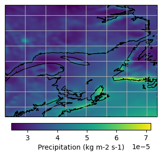
We then subset the data for a zone and period of interest, namely eastern Canada for the period 1981-2010, using clisops subset_bbox function. We also demonstrate how to select a single grid cell according to its longitude and latitude using clisops subset_gridpoint. Note that we can’t simply use xarray’s sel method here because dimensions are in rotated pole coordinates.

Other, and more advanced subsetting capabilities are also available. For more information and examples, consult those subsetting examples.

from clisops.core import subset
from matplotlib import pyplot as plt

# Subset bounding box
lon_bnds = [-70, -55]
lat_bnds = [44, 55]

# Loading the coordinate data speeds up the subsetting process a little
for coord in ["lat", "lon"]:
    ds[coord] = ds[coord].load()

# Subset bbox
bbox = subset.subset_bbox(
    ds, lon_bnds=lon_bnds, lat_bnds=lat_bnds, start_date="1981", end_date="2010"
)

# Subset gridpoint
site = subset.subset_gridpoint(ds, lat=40, lon=-60)

with xr.set_options(display_expand_data_vars=False, display_expand_coords=False):
    display(bbox)
    display(site)

<xarray.Dataset> Size: 45GB
Dimensions:       (rlat: 156, rlon: 150, time: 10957)
Coordinates: (6)
Data variables: (49)
Attributes: (12/30)
    Conventions:             CF-1.8
    Remarks:                 Original variable names are following the conven...
    contact:                 
    doi:                     https://doi.org/10.5194/hess-25-4917-2021
    domain:                  NAM
    frequency:               day
    ...                      ...
    history:                 2025-12-16 11:21:02.543093: Created a copy of Ca...
    description:             Original data source: https://hpfx.collab.scienc...
    institute:               Environment and Climate Change Canada
    institute_id:            ECCC
    dataset_description:     https://hpfx.collab.science.gc.ca/~scar700/rcas-...
    dataset_id:              CaSRv3.2

<xarray.Dataset> Size: 3MB
Dimensions:       (time: 16437)
Coordinates: (6)
Data variables: (49)
Attributes: (12/30)
    Conventions:             CF-1.8
    Remarks:                 Original variable names are following the conven...
    contact:                 
    doi:                     https://doi.org/10.5194/hess-25-4917-2021
    domain:                  NAM
    frequency:               day
    ...                      ...
    history:                 2025-12-16 11:21:02.543093: Created a copy of Ca...
    description:             Original data source: https://hpfx.collab.scienc...
    institute:               Environment and Climate Change Canada
    institute_id:            ECCC
    dataset_description:     https://hpfx.collab.science.gc.ca/~scar700/rcas-...
    dataset_id:              CaSRv3.2

Data analysis¶

Here we’ll compute the 10-year precipitation average on the eastern Canada subset using dask to parallelize computations. A dictionary of options is given to dask to specify the number of workers, threads per worker, memory limit, etc.

# NBVAL_IGNORE_OUTPUT

import logging

from dask.distributed import Client
from IPython.display import clear_output

# For hourly data, we suggest using the following chunking pattern: dict(time=720, rlon=50, rlat=50)
# Compute 10-year precipitation means. This is a lazy operation, no computations are done at this point.
pr10y = bbox.pr.resample(time="10YS").mean(dim="time", keep_attrs=True)

# Options for dask workers
dask_kwargs = dict(
    n_workers=8,
    threads_per_worker=6,
    memory_limit="2.5GB",
    local_directory="/notebook_dir/writable-workspace/tmp",
    silence_logs=logging.ERROR,
)

# Actually perform the computation
with Client(**dask_kwargs) as c:
    clear_output()
    display(c)
    # Just taking the first 10-year average to speed things up
    pr10y = pr10y.isel(time=0).compute()
clear_output()
pr10y.plot()

<matplotlib.collections.QuadMesh at 0x7f1cb1dffda0>

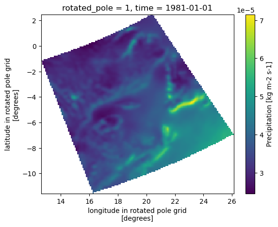
../_images/d996ca56776d8570f812e8177fe58b969b8bc07f63d2ff341cbaddd5f281587c.png

Note that the graphic axes follow the dimensions of the dataset, namely rotated longitudes and latitudes. The bounding box subset is however performed on longitudes and latitudes, and the areas outside of the bounding box are filled with NaNs, which explain the presence of white areas in the graph.

In this second example, we’ll use xclim to compute the heat index’ annual maxima at the selected site. The heat index accounts for both temperature and relative humidity to describe human perception of heat.

# NBVAL_IGNORE_OUTPUT

from xclim import convert

# Compute heat index using xclim and find the annual maxima.
with Client(**dask_kwargs) as c:
    clear_output()
    display(c)
    hi_max = convert.heat_index(ds=site).resample(time="Y").max()
clear_output()

# Plot the results
hi_max.plot()

[<matplotlib.lines.Line2D at 0x7f1c9b235220>]

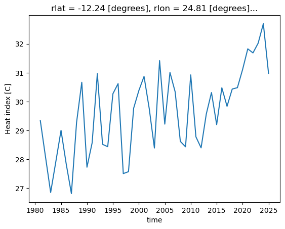
../_images/c2af243e7aff4fae384e36cb720b01798955b9a9800ff427f91b6affe7a24cce.png

Visualization¶

Finally, we show how plot the CaSR data on a map. We need to specify two projections: one for the map, and another for the data. The Cartopy library is then able to connect data coordinates to map coordinates.

Here for simplicity we’ll use the regular lat-lon projection, called PlateCarree. Other choices would be Orthographic for a remote sensing view of the Earth, or LambertConformal, a projection often used for Canada-wide maps.

The details of the data coordinate reference system are stored for convenience within the rotated_pole variable’ attributes.

bbox.rotated_pole

<xarray.DataArray 'rotated_pole' ()> Size: 4B
array(1, dtype=int32)
Coordinates:
    rotated_pole  int32 4B 1
Attributes:
    north_pole_grid_longitude:  0.0
    grid_north_pole_latitude:   31.758312454493154
    grid_north_pole_longitude:  87.59703130293302
    earth_radius:               6370997.0
    grid_mapping_name:          rotated_latitude_longitude

import cartopy.crs as ccrs

# A regular lat-lon projection for the map
pc = ccrs.PlateCarree()

# The coordinate reference system for the rotated pole data
rotp = ccrs.RotatedPole(
    pole_longitude=bbox.rotated_pole.grid_north_pole_longitude,
    pole_latitude=bbox.rotated_pole.grid_north_pole_latitude,
)

# Plot rotated pole data on a regular lat lon grid.
fig = plt.figure(figsize=(4, 4))

# Here we specify the map projection
ax = plt.subplot(1, 1, 1, projection=pc)
ax.set_extent(lon_bnds + lat_bnds)

# Here we specify the transformation required to map data coordinates to map coordinates.
m = ax.pcolormesh(pr10y.rlon, pr10y.rlat, pr10y, transform=rotp)

# Fine-tuning
ax.coastlines()
ax.gridlines()
plt.colorbar(
    m,
    orientation="horizontal",
    label=f"{pr10y.long_name} ({pr10y.units})",
    fraction=0.046,
    pad=0.04,
)

<matplotlib.colorbar.Colorbar at 0x7f1c9aebd4f0>

../_images/5de09a3e01a7f5acd5b835203e13f6799bc3d9caddea8c3b70817cbfcc406730.png