Programmatic access to geospatial layers from the deca-millennial flood project

The relative and absolute changes in 1,000 and 10,000 flood frequency values have been computed for over 500 watersheds using two climate projection large ensembles, CESM1 and CanESM2 (see project overview for more info). These results are available on the PAVICS GeoServer, and this notebook shows how to get access to those files from a programming environment.

%matplotlib inline

import json

import geopandas as gpd
from owslib.wfs import WebFeatureService

# Connect to Ouranos' GeoServer WFS service.
url = "https://pavics.ouranos.ca/geoserver/wfs"
wfs = WebFeatureService(url, version="2.0.0")

typename = "public:decamillenial_flood_CC"
layer = wfs.contents[typename]
print(layer.abstract)

Climate change factors for 1,000 and 10,000-year design floods estimated from the CESM1 and CanESM2 Large Ensembles and the GR4J-Cemaneige hydrological model over the period 2080-2100 compared to 1990-2010.

In the next cell, we’ll download the data in the GeoJSON format, load it into a dictionary and instantiate a GeoDataFrame.

typename = "public:decamillenial_flood_CC"
txt = wfs.getfeature(typename=typename, outputFormat="json").read()
data = json.loads(txt.decode())
gdf = gpd.GeoDataFrame.from_features(data)

Let’s take a look at the top of the table.

gdf.head()

	geometry	ID	name	watershed_area	NSE	CESM1_PWM_T100_MUL	CESM1_PWM_T100_P75_MUL	CESM1_PWM_T100_P90_MUL	CESM1_PWM_T100_P95_MUL	CESM1_PWM_T100_P99_MUL	...	CanESM2_PWM_T1000_ADD	CanESM2_PWM_T1000_P75_ADD	CanESM2_PWM_T1000_P90_ADD	CanESM2_PWM_T1000_P95_ADD	CanESM2_PWM_T1000_P99_ADD	CanESM2_PWM_T10000_ADD	CanESM2_PWM_T10000_P75_ADD	CanESM2_PWM_T10000_P90_ADD	CanESM2_PWM_T10000_P95_ADD	CanESM2_PWM_T10000_P99_ADD
0	POLYGON ((-111.39170 54.17100, -111.42500 54.1...	06CD002	CHURCHILL RIVER ABOVE OTTER RAPIDS	119000.0	0.715358	-57.343822	-54.547526	-51.714055	-49.651469	-46.376278	...	-0.274774	-0.220550	-0.162439	-0.128182	-0.068190	-0.138914	-0.022957	0.136653	0.224204	0.422348
1	POLYGON ((-134.94580 59.57930, -134.80000 59.6...	09AA014	FANTAIL RIVER AT OUTLET OF FANTAIL LAKE	717.0	0.758993	27.442331	31.577337	35.676450	38.155664	43.461187	...	3.627438	5.299869	7.212052	8.076060	10.182767	1.583382	5.487793	9.107839	11.806705	15.833487
2	POLYGON ((-130.19170 59.40850, -130.17920 59.4...	10AC004	BLUE RIVER NEAR THE MOUTH	1700.0	0.818958	8.734342	13.139980	17.049680	19.928544	24.816201	...	4.524804	5.183105	6.138951	6.809163	7.634194	9.541766	11.049454	13.842788	15.958528	18.720224
3	POLYGON ((-126.10000 58.79600, -126.11250 58.8...	10BE007	TROUT RIVER AT KILOMETRE 783.7 ALASKA HIGHWAY	1170.0	0.846326	1.782831	6.310975	10.423199	13.551472	17.247709	...	-0.826701	0.289358	1.253341	1.857471	2.806194	-2.461317	-0.095001	1.757461	3.090589	4.684330
4	POLYGON ((-130.50830 58.44600, -130.52500 58.4...	10AC003	DEASE RIVER AT OUTLET OF DEASE LAKE	1520.0	0.961293	12.827155	17.025618	20.555976	22.540481	26.720056	...	2.612100	3.271549	3.910924	4.246732	4.884688	3.814419	5.089299	6.404652	7.192629	7.993150

5 rows × 65 columns

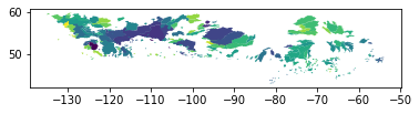
And let’s create a basic plot for the values of one of the columns, here the relative change factor for the 100-year event estimated from the CanESM2 Large Ensemble, using the Probability Weighted Moment method to estimate GEV parameters.

col = "CanESM2_PWM_T100_MUL"
gdf.plot(column=col)

<Axes: >