Working with owslib’s WMS interface

OWSlib is a Python package for client programming with OGC web service interface standards. In this tutorial we’ll work with the WMS interface.

from owslib.wms import WebMapService

Web Mapping Service

We start by fetching a map using the WMS protocol. We first instantiate a WebMapService object using the address of the NASA server, then browse through its content.

wms = WebMapService("https://neo.gsfc.nasa.gov/wms/wms")
print("Title: ", wms.identification.title)
print("Type: ", wms.identification.type)
print("Operations: ", [op.name for op in wms.operations])
print("GetMap options: ", wms.getOperationByName("GetMap").formatOptions)
wms.contents.keys()

Traceback (most recent call last):

  File ~/checkouts/readthedocs.org/user_builds/pavics-sdi/conda/latest/lib/python3.10/site-packages/IPython/core/interactiveshell.py:3577 in run_code
    exec(code_obj, self.user_global_ns, self.user_ns)

  Cell In[2], line 1
    wms = WebMapService("https://neo.gsfc.nasa.gov/wms/wms")

  File ~/checkouts/readthedocs.org/user_builds/pavics-sdi/conda/latest/lib/python3.10/site-packages/owslib/wms.py:50 in WebMapService
    return wms111.WebMapService_1_1_1(

  File ~/checkouts/readthedocs.org/user_builds/pavics-sdi/conda/latest/lib/python3.10/site-packages/owslib/map/wms111.py:74 in __init__
    self._capabilities = reader.read(self.url, timeout=self.timeout)

  File ~/checkouts/readthedocs.org/user_builds/pavics-sdi/conda/latest/lib/python3.10/site-packages/owslib/map/common.py:69 in read
    return etree.fromstring(raw_text)

  File src/lxml/etree.pyx:3264 in lxml.etree.fromstring

  File src/lxml/parser.pxi:1989 in lxml.etree._parseMemoryDocument

  File src/lxml/parser.pxi:1876 in lxml.etree._parseDoc

  File src/lxml/parser.pxi:1164 in lxml.etree._BaseParser._parseDoc

  File src/lxml/parser.pxi:633 in lxml.etree._ParserContext._handleParseResultDoc

  File src/lxml/parser.pxi:743 in lxml.etree._handleParseResult

  File src/lxml/parser.pxi:672 in lxml.etree._raiseParseError

  File <string>:1
XMLSyntaxError: Start tag expected, '<' not found, line 1, column 1

The content is a dictionary holding metadata for each layer. We’ll print some of the metadata’ title for a couple of layers to see what’s in it.

for key in [
    "MOD14A1_M_FIRE",
    "CERES_LWFLUX_M",
    "ICESAT_ELEV_G",
    "MODAL2_M_CLD_WP",
    "MOD_143D_RR",
]:
    print(wms.contents[key].title)

Active Fires (1 month - Terra/MODIS)
Outgoing Longwave Radiation (1 month)
Greenland / Antarctica Elevation
Cloud Water Content (1 month - Terra/MODIS)
True Color (1 day - Terra/MODIS)

We’ll select the true color Earth imagery from Terra/MODIS. Let’s check out some of its properties. We can also pretty print the full abstract with HTML.

# NBVAL_IGNORE_OUTPUT

from IPython.core.display import HTML

name = "MOD_143D_RR"
layer = wms.contents[name]
print("Abstract: ", layer.abstract)
print("BBox: ", layer.boundingBoxWGS84)
print("CRS: ", layer.crsOptions)
print("Styles: ", layer.styles)
print("Timestamps: ", layer.timepositions)
HTML(layer.parent.abstract)

Abstract:  None
BBox:  (-180.0, -90.0, 180.0, 90.0)
CRS:  ['EPSG:4326']
Styles:  {}
Timestamps:  ['2006-09-01/2006-09-14/P1D', '2006-09-17/2006-10-10/P1D', '2006-10-12/2006-11-18/P1D', '2006-11-21/2007-08-16/P1D', '2007-08-18', '2007-08-20/2007-09-11/P1D', '2007-09-15/2007-12-30/P1D', '2008-01-01/2008-06-12/P1D', '2008-06-14', '2008-06-16/2008-07-12/P1D', '2008-07-14/2008-09-17/P1D', '2008-09-19', '2008-09-22/2008-10-17/P1D', '2008-10-19/2008-10-22/P1D', '2008-10-28/2008-12-02/P1D', '2008-12-04/2008-12-20/P1D', '2008-12-23/2008-12-30/P1D', '2009-01-01/2009-01-20/P1D', '2009-01-22/2009-04-19/P1D', '2009-04-23/2009-07-05/P1D', '2009-07-08/2009-12-30/P1D', '2010-01-01/2010-07-16/P1D', '2010-07-18/2010-12-07/P1D', '2010-12-09/2010-12-30/P1D', '2011-01-01/2011-01-25/P1D', '2011-01-27/2011-03-19/P1D', '2011-03-21/2011-07-23/P1D', '2011-07-27/2011-08-27/P1D', '2011-08-30/2011-12-13/P1D', '2011-12-15/2012-02-19/P1D', '2012-02-21/2013-12-01/P1D', '2013-12-04/2018-03-12/P1D', '2018-03-14/2018-05-16/P1D', '2018-05-18/2018-09-17/P1D', '2018-09-19/2022-05-04/P1D', '2022-05-06/2022-12-21/P1D', '2022-12-23/2023-09-28/P1D', '2023-10-01/2023-10-17/P1D']

These images show the Earth's surface and clouds in true color, like a photograph. NASA uses satellites in space to gather images like these over the whole world every day. Scientists use these images to track changes on Earth's surface. Notice the shapes and patterns of the colors across the lands. Dark green areas show where there are many plants. Brown areas are where the satellite sensor sees more of the bare land surface because there are few plants. White areas are either snow or clouds. Where on Earth would you like to explore?

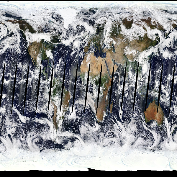
Getting the image data

Now let’s get the image ! The response we’re getting is a ResponseWrapper object, we need to read its content to get the actual bytes for the png file. Let’s first display the raw image, then try to map it onto a projection of the Earth.

response = wms.getmap(
    layers=[
        name,
    ],
    styles=["rgb"],
    bbox=(-180, -90, 180, 90),  # Left, bottom, right, top
    format="image/png",
    size=(600, 600),
    srs="EPSG:4326",
    time="2018-09-16",
    transparent=True,
)
response

<owslib.util.ResponseWrapper at 0x7fa543b4fdf0>

from IPython.display import Image

Image(response.read())

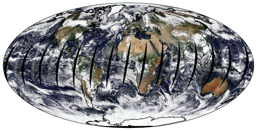
Plotting the image on a map

Using the cartopy library, we’ll overlay the image on a map of the Earth. Since Matplotlib’s imread function expects a file-like object, we’ll mimic a file object in memory using the io.BytesIO function.

import io
import warnings

import cartopy
import matplotlib.pyplot as plt

image = io.BytesIO(response.read())
data = plt.imread(image)

warnings.filterwarnings("ignore", category=cartopy.io.DownloadWarning)
fig = plt.figure(figsize=(8, 6))
ax = fig.add_axes([0, 0, 1, 1], projection=cartopy.crs.Mollweide())
ax.imshow(
    data,
    origin="upper",
    extent=(-180, 180, -90, 90),
    transform=cartopy.crs.PlateCarree(),
)
ax.coastlines()
plt.show()